In quantitative fluorescence microscopy, we assume that the pixel intensity is proportional to the concentration of the fluorophore. However, uneven illumination (vignetting) and optical obstructions (dust) violate this assumption. Without correction we may have (1) Intensity bias, where cells may appear brighter in the middle than on the edge, (2) Segmentation errors segmentation algorithms may fail in certain part of an image. Therefore it is important to learn methods on how to mitigate illumination artefatcs.
Prerequisites
Before starting this lesson, you should be familiar with:
After completing this lesson, learners should be able to:
Formulate the mathematical relationship between the raw image and the corrected image
Evaluate methods to obtain a flat-field reference (calibration slide or retrospective computation)
Perform a flat-field correction and evaluate the results
Concept map
graph TD
S("Sample img. (S)")
B("Dark frame (D)")
Slide["Standard slide/dye"] --- F("Bright img. (F)")
Retrospective["Restrospective Mean/Median"] --- F
S --- Subtraction(("Subtract D"))
B --- Subtraction
F --- Subtraction
subgraph math[" "]
Subtraction --- S_bg("S background corr. (Sb)")
Subtraction --- F_bg("F background corr. (Fb)")
F_bg --- Normalization(("NormalizeFb/mean(Fb)"))
Normalization --- F_bg_norm("Flat field reference (Ff)")
F_bg_norm --- Division
S_bg --- Division(("Divide Sb/Ff"))
%% Bottom label simulation
L["Math Operations"]
style L fill:none,stroke:none,font-weight:bold
end
Division --- Corrected("Flat field corrected sample image")
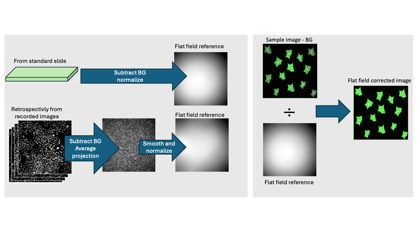
Figure
Left side - To compute a flat field reference we can use a measurement from a standard (homgeneous) slide or retrospectively use acquired images. Right side - Given a flat-field reference we can perform the correction of the illumination aberration
To perform a flat field correction we need to first compute a normalized flat field that can be used to correct
the images acquired with the same modality. For this one can record an homogeneous fluorescent slide and then perform
background subtraction and normalization. The resulting image will have values around 1. Make sure that you work
with the correct bit-depth (32-bit or more) to account for real numbers.
run("Close All");// Compute the normalized flat field// load a bright homogeneous image (standard slide)open("https://github.com/NEUBIAS/training-resources/raw/master/image_data/shading_tiling/xy_16bit__homogeneous_slide.tif");rename("bright_image");// load the camera background// Drag and dropopen("https://github.com/NEUBIAS/training-resources/raw/master/image_data/shading_tiling/xy_16bit__bg_camera.tif");// [Image › Rename...]rename("camera_bg");// Subtract the camera background// [Process › Image Calculator...]imageCalculator("Subtract create 32-bit","bright_image","camera_bg");// Smooth the result to remove noise// [Process › Filters › Gaussian Blur...]run("Gaussian Blur...","sigma=50");//Compute the mean value and normalize// Make sure the that you can measure the meanrun("Set Measurements...","area mean display redirect=None decimal=3");// [ Analyze › Clear Results]run("Clear Results");// [ Analyze › Measure]run("Measure");// Copy value of mean m=getResult("Mean",0);// Perform normalization // [Process › Math › Divide...]run("Divide...","value="+m);// [Image › Rename...]rename("flat_field_normalized");run("Enhance Contrast","saturated=0.35");
Given that we have normalized flat-field we can correct any image that has been recorded with same
modality (objective, ligh-source). We computed the flat-field in the previous activity.
Make sure that you work with the correct bit-depth (32-bit or more) to account for real numbers.
Divide the background subtracted sample image by the normalized flat field
Show activity for:
ImageJ Macro
run("Close All");// Load image where we want to apply a flat field correction open("https://github.com/NEUBIAS/training-resources/raw/master/image_data/shading_tiling/xyc_16bit__hoechst_phalloidin_tile_01.tif");rename("sample_img");// load the camera background// Drag and dropopen("https://github.com/NEUBIAS/training-resources/raw/master/image_data/shading_tiling/xy_16bit__bg_camera.tif");// [Image › Rename...]rename("camera_bg");// Subtract the camera backgroundimageCalculator("Subtract create 32-bit stack","sample_img","camera_bg");rename("sample_img_bg_corr");// load the normalized flat-field// Drag and dropopen("https://github.com/NEUBIAS/training-resources/raw/master/image_data/shading_tiling/xy_32bit__flat_field.tif");rename("flat_field_normalized");run("Enhance Contrast","saturated=0.35");// Flat field correctionimageCalculator("Divide create 32-bit stack","sample_img_bg_corr","flat_field_normalized");rename("sample_img_flat_field_corr");run("Enhance Contrast","saturated=0.35");run("Tile");
Often we can’t record a standard image or it may not reflect our sample peculiarities.
In this case if we have enough images we can compute an approximate flat field. A typical operation is to compute an average of all images followed by smoothing.
Make sure that you work with the correct bit-depth (32-bit or more) to account for real numbers.
Load the a stack of images xy_16bit__hoechst_downsampled_stack.tif. These images have been acquired at several positions and then stacked together for convenience in a single file.
Perform a smoothing using for example a gaussian up to the field become homogeneous
Normalize the obtained image by its mean
Show activity for:
ImageJ Macro
run("Close All");// Open images of hoechst// These are several positions stacked as a "Z-stack"open("https://github.com/NEUBIAS/training-resources/raw/master/image_data/shading_tiling/xy_16bit__hoechst_downsampled_stack.tif");rename("stack");// Open the camera backgroundopen("https://github.com/NEUBIAS/training-resources/raw/master/image_data/shading_tiling/xy_16bit__bg_camera_downsampled.tif");rename("camera_bg");// We subtract the camera background and the result is converted to 32 bit - Important for subsequent normalizationimageCalculator("Subtract create 32-bit stack","stack","camera_bg");rename("stack_bg_corrected");// Compute an average imagerun("Z Project...","projection=[Average Intensity]");// Smooth the image to obtain an homogeneous fieldrun("Gaussian Blur...","sigma=50");rename("flat_field_unnormalized");run("Duplicate...","title=flat_field_normalized");//Compute the mean value and normalizerun("Clear Results");run("Measure");m=getResult("Mean",0);run("Divide...","value="+m);run("Enhance Contrast","saturated=0.35");
Assessment
Which of the following issues can be corrected using a standard Flat-field correction (FFC)?
Random Poisson noise (shot noise)
Uneven illumination and dust on the lens
Over-saturated pixels
Specimen movement during acquisition
Solution
Issue number 2
What is the primary purpose of a “Dark Frame” (or Background Reference) in the FFC workflow?
To measure the maximum brightness of the lamp.
To identify the focal plane.
To subtract the electronic signal generated by the sensor in the absence of light (Dark Current/Offset).
To normalize the image to 1.0.
Solution
Answer number 3
You change your microscope objective from 10x to 40x. Can you use the same flat-field reference image?
Yes, the illumination pattern is independent of the objective.
No, the optical path and shading patterns are specific to each objective/filter combination.