Illumination and shading artefacts


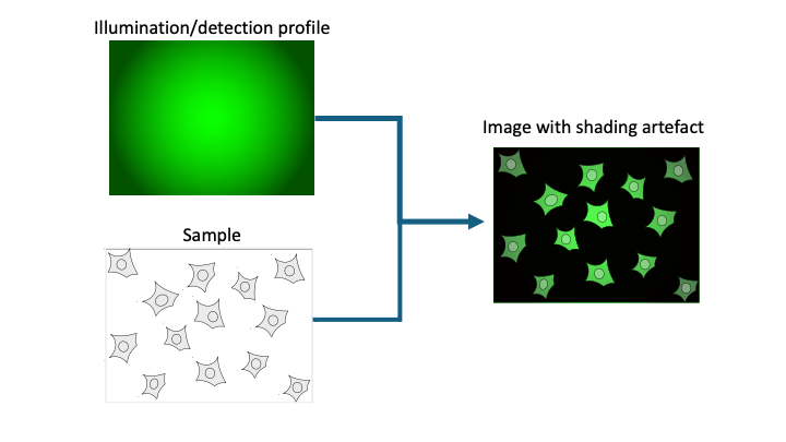
Non-uniform illumination and shading artefacts are common image quality issues where brightness varies unevenly across an image, often appearing as vignetting (darker corners), streaks, or gradient shadows. These effects arise from lighting inefficiencies, detection limitations, and/or light path obstructions. They degrade the image quality and confuse intensity-based analysis and image processing.


Prerequisites

Before starting this lesson, you should be familiar with:

Learning Objectives

After completing this lesson, learners should be able to:
  • Identify global shading patterns caused by e.g. Gaussian illumination

  • Understand implication for intensity measurements

Concept map

flowchart TD S("Sample") --> |Illumination/detection| I("Image") LS("Light Source (Gaussian)") --> A("Illumination artefacts") OP("Optical Path (Dust/Dirt)") --> A AL("Misalignment (Köhler)") --> A A --> Vignetting("Vignetting (Bright Center)") A --> Gradient("Intensity Gradient") A --> Shadows("Shadows") A --> More("...")

Figure


Uneven illumination creates artefacts in the image


Activities

Inspect shading artefact in a fluorescence image

Open these images, cells stained for their nuclei (Hoechst, 1st channel) and actin (phalloidin, 2nd channel):

Do you notice a pattern of intensity difference from the center to the corner in all images? How does this affect your intensity measurements?

Open xy_16bit__homogeneous_slide.tif. This image has been recorded with a an homogeneous fluorescent slide on the same setup. Show how the intensity pattern matches the pattern observed when measuring the biological sample. The intensity pattern is a typical pattern observed in widefield system and gaussian illumination.


Show activity for:  

ImageJ GUI

Inspect shading artefact in a fluorescence image

  • Drag and drop xyc_16bit__hoechst_phalloidin_tile_01.tif to ImageJ
  • Draw a line across the diagonal of the image, if possible increase the width of the line to 50 pixels (this makes the graph more clear)
  • Plot a profile Ctrl-K [Analyze › Plot Profile]
  • Press Live in the Plot window
  • Change between channels and also on different lines across the image
  • You should notice a difference in intensities between the center and border of the image?
  • Drag and drop xyc_16bit__hoechst_phalloidin_tile_02.tif to ImageJ
  • Repeat the operation and show that one has a similar result
  • Drag and drop xy_16bit__homogeneous_slide.tif to ImageJ
  • Discuss the pattern and how it matches what is observed with the biological sample

ImageJ macro

// Close all images
run("Close All")

// Open the first image 
open("https://github.com/NEUBIAS/training-resources/raw/master/image_data/shading_tiling/xyc_16bit__hoechst_phalloidin_tile_01.tif")
makeLine(50, 50, 2250, 2250);
run("Plot Profile");

// Open the first image 
open("https://github.com/NEUBIAS/training-resources/raw/master/image_data/shading_tiling/xyc_16bit__hoechst_phalloidin_tile_02.tif")
makeLine(50, 50, 2250, 2250);
run("Plot Profile");

// Open the slide image
open("https://github.com/NEUBIAS/training-resources/raw/master/image_data/shading_tiling/xy_16bit__homogeneous_slide.tif")
makeLine(50, 50, 2250, 2250);
run("Plot Profile");


Follow-up material

Recommended follow-up modules:

Learn more: