Images are a collection of a lot (millions) of values, which is information that is hard to process for our human brains. Thus, one typically assigns a color to each distinct value, by means of a lookup table (LUT). There is no fix recipe for how to adjust this mapping from numbers to colors. It is easy to chose a mapping that hides certain information in an image, while emphasising other information. Thus, configuring this mapping properly is a great responsibility that scientists have to take on when presenting their image data.
Prerequisites
Before starting this lesson, you should be familiar with:
After completing this lesson, learners should be able to:
Understand how the numerical values in an image are transformed into colourful images.
Understand what a lookup table (LUT) is and how to adjust it.
Appreciate that choosing the correct LUT is a very serious responsibility when preparing images for a talk or publication.
Concept map
graph TD
V("Image pixel value") --> L("Lookup table (LUT)")
L --> |does not change|V
L --> |changes|C("Displayed pixel color & brightness")
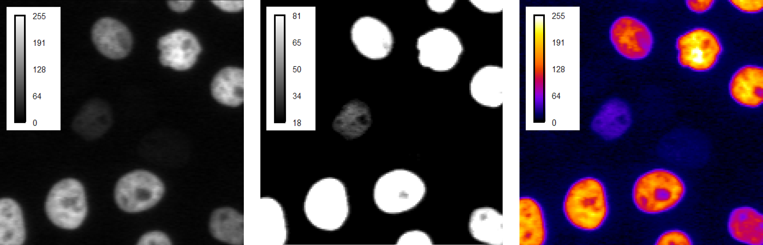
Figure
Left: Image displayed with a grey LUT and the color mapping as an inset. Right: Image shown with several different LUTs.
Lookup tables do the mapping from a numeric pixel value to a color. This is the main mechanism how we visualise microscopy image data. In case of doubt, it is always a good idea to show the mapping as an inset in the image (or next to the image).
Single color lookup tables
Single color lookup tables are typically configured by chosing one color such as, e.g., grey or green, and choosing a min and max value that determine the brightness of this color depending on the value of the respective pixel in the following way:
brightness( value ) = ( value - min ) / ( max - min )
In this formula, 1 corresponds to the maximal brightness and 0 corresponds to the minimal brightness that, e.g., your computer monitor can produce.
Depending on the values of value, min and max it can be that the formula yields values that are less than 0 or larger than 1.
This is handled by assinging a brightness of 0 even if the formula yields values < 0 and assigning a brightness of 1 even if the formula yields values
larger than 1. In such cases one speaks of “clipping”, because one looses (“clips”) information about the pixel value (see below for an example).
Both pixel values will be painted with the same brightness as a brightness larger than 1 is not possible (see above).
Multi color lookup tables
As the name suggestes multi color lookup tables map pixel gray values to different colors.
For example:
0 -> black
1 -> green
2 -> blue
3 -> ...
Typical use cases for multi color LUTs are images of a high dynamic range (large differences in gray values) and label mask images (where the pixel values encode object IDs).
Sometimes, also multi color LUTs can be configured in terms of a min and max value. The reason is that multi colors LUTs only have a limited amount of colors, e.g. 256 different colors. For instance, if you have an image that contains a pixel with a value of 300 it is not immediately obvious which color it should get; the min and max settings allow you to configure how to map your larger value range into a limited amount of colors.
To visualize an image there are several lookup tables to choose from.
Depending on the use-case, one can be more appropriate than another.
In this activity, we will look at commonly used LUTs and discuss how and when to use them.
# %%
# Using different Lookup Tables (LUTs) in napari
# %%
# Instantiate the napari viewer
importnapariviewer=napari.Viewer()# %%
# Read an image and its metadata
fromOpenIJTIFFimportopen_ij_tiffimage,*_=open_ij_tiff("https://github.com/NEUBIAS/training-resources/raw/master/image_data/xy_8bit__nuclei_high_dynamic_range.tif")# %%
# Add the image
viewer.add_image(image)# %%
# Napari:
# Right click on "contrast limits" and adjust to see the dim nuclei
# Set "colormap" to "turbo" and change the contrast limits back to 0, 255
# Appreciate the such a multi-color LUT can be useful to see dim and bright objects
# %%
# Programatically show the image several times with different LUT settings
viewer.layers.clear()# remove all layers
viewer.add_image(image,name="image_turbo",colormap="turbo",contrast_limits=[0,255])viewer.add_image(image,name="image_gray_1",colormap="gray",contrast_limits=[0,100])viewer.add_image(image,name="image_gray_2",colormap="gray",contrast_limits=[0,255])viewer.grid.enabled=True# turn on the grid mode to see the images side by side
# %%
# Close the viewer (CI test requires this)
viewer.close()
Paste the image url: https://github.com/NEUBIAS/training-resources/raw/master/image_data/xy_8bit__nuclei_high_dynamic_range.tif and click the Start button
Click the Close button after upload finishes, then the image will be available in your Galaxy history.
Start the Napari Interactive Tool
In the Tools panel on the left, search for Run Napari interactive tool
Select xy_8bit_nuclei_high_dynamic_range.tif from the Images dropdown list.
Click the Run Tool button. Once the Open link appears at the top of the page, click it to open Napari in a separate browser tab.
In the Napari browser tab, navigate to File -> Open File(s) and select the image xy_8bit_nuclei_high_dynamic_range.tif from the input folder.
Change the Contrast settings
Experiment with different minimum and maximum values of the contract limits.
Notice how, at certain settings, a very dim nucleus becomes visible.
Explore different LUTs, e.g.
Go to File › Open File(s)
Select the same image xy_8bit_nuclei_high_dynamic_range.tif from the input folder. A new layer will appear in the bottom left pane.
Change the colormap to turbo, from the layer options in the top left pane.
Turn on grid mode by clicking the Grid button located at the bottom left,second from the right.
Very often, one has a set of images that represent different biological conditions and that have been acquired with the same microscopy settings. In order to be able to judge whether there is a difference between the biologic conditions, it is critical to display them with the same color mapping settings.
In this activity, we will explore important ways how to achieve such comparable visualisation:
Display image sets with the same color map and the same contrast settings
# %%
# Show two images with the same LUT settings
# %%
# Instantiate the napari viewer
importnapariviewer=napari.Viewer()# %%
# Read the images
fromOpenIJTIFFimportopen_ij_tiffimage_control,*_=open_ij_tiff('https://github.com/NEUBIAS/training-resources/raw/master/image_data/xy_calibrated_16bit__nuclear_protein_control.tif')image_treated,*_=open_ij_tiff('https://github.com/NEUBIAS/training-resources/raw/master/image_data/xy_calibrated_16bit__nuclear_protein_treated.tif')# %%
# View the image as grayscale
viewer.add_image(image_control,name='control',colormap='gray')viewer.add_image(image_treated,name='treated',colormap='gray')# %%
# Napari: Toggle grid mode on to the see images side by side
# Napari: Check the contrast limits for the two images
# %%
# Check the contrast limits programatically
print(viewer.layers['control'].contrast_limits)print(viewer.layers['treated'].contrast_limits)# %%
# Apply the same contrast to both images
viewer.layers['control'].contrast_limits=(0,2500)viewer.layers['treated'].contrast_limits=(0,2500)# %%
# Close the viewer (CI test requires this)
viewer.close()
Galaxy Napari
Upload one of the above pairs of images to Galaxy
Go to https://usegalaxy.eu
In the Tools panel on the left, click Upload Data
Click Paste/Fetch data button
Paste the URLs of the two images(one line per URL) and click the Start button
Click the Close button after upload finishes, then the image will be available in your Galaxy history.
Start the Napari interactive tool
In the Tools panel on the left, search for Run Napari interactive tool
Select the two uploaded images from the Images dropdown list
Click the Run Tool button. Once the Open link appears at the top of the page, click it to open Napari in a separate browser tab.
In the Napari tab, navigate to File -> Open file(s), and select the two images from the input folder.
Turn on grid mode by clicking the Grid button located at the bottom left,second from the right. The two images will appear side by side
Adjust the contrast limits and apply the same values to both images to compare them directly
Assessment
Compute how the contrast limits affect the rendered pixel brightness
Read the below section “Explanations: Single color lookup tables” and use the formula that is given there to compute the rendered pixel brightness for the following scenarios:
value = 49, min = 10, max = 50, brightness = ?
value = 100, min = 0, max = 65, brightness = ?
value = 10, min = 20, max = 65, brightness = ?
Solution
0.975
1.538 -> 1.0
-0.22 -> 0.0
Fill in the blanks
Fill in the blanks using those words: larger than, smaller than
Pixels with values _____ max will appear saturated.
Pixels with values _____ the min will appear black (using a single color LUT).
Solution
larger than
smaller than
Key points
LUT stands for “look-up table”; it defines how numeric pixel values are mapped to colors for display.
A LUT has configurable contrast limits that determine the pixel value range that is rendered linearly.
LUT settings must be responsibly chosen to convey the intended scientific message and not to hide relevant information.
A gray scale LUT is usually preferable over a colour LUT, especially blue and red are not well visible for many people.
For high dynamic range images multi-color LUTs may be useful to visualise a wider range of pixel values.