Apart from the X and Y dimensions, visible in the width and height of an image, image data can have additional dimensions. The most common additional dimensions include:
the Z dimension, providing depth to image data,
different channels, showing data recorded with different detectors or detector settings,
the time dimension.
Viewing multi-dimensional data can be challenging, because a computer monitor can only render a (multi-color) 2D representation. Therefore, it is important to know how to visualize and navigate through multi-dimensional data.
Prerequisites
Before starting this lesson, you should be familiar with:
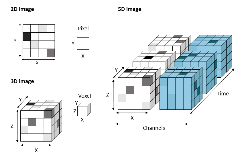
Schematic representation of 2D, 3D, and 5D image data. 2D images are made up of tiny squares called pixels, whereas 3D images are made up of cubes called voxels.
Observe that the image has 3 dimensions, X, Y, and Z.
Explore the different dimensions using [ Image > Stacks > Orthogonal Views ] or [Ctrl-Shift-H].
Explore the effect of wrong calibration:
Open image properties: [ Image > Properties… ] or [Ctrl-Shift-P].
Change all dimensions to 1 pixel.
Observe that the cell now appears as an oval in the Orthogonal Views.
Reopen the image in order to have the correct calibration.
Napari GUI/Python
Open the 3D image xyz_8bit__chromsomes.tif by dragging and dropping the file in a Napari viewer.
The data shows chromosomes wrapped around a nucleus, but it does not appear spherical.
View the data in XY, YZ, and XZ by rotating the stack (third button in the bottom left corner) and by activating the 3D-view option (second button in the bottom left corner).
Observe that the image is not calibrated, because the XZ and YZ views are deformed and the chromosomes are wrapped around a nucleus that should be spherical but does not appear so in the image.
To take the calibration into account, open the console (first button in the bottom left corner: >_) and type viewer.layers[0].scale = (0.1500000, 0.0338542, 0.0338542). Observe the difference in the 3D view.
skimage napari
# %%
# Explore a 3D image
# %%
# Imports
fromOpenIJTIFFimportopen_ij_tifffromnapari.viewerimportViewer# %%
# Load the image
image,axes,scales,units=open_ij_tiff("https://github.com/NEUBIAS/training-resources/raw/master/image_data/xyz_8bit__chromosomes.tif")# View the image in napari
viewer=Viewer()viewer.add_image(image)# [markdown]
# Napari GUI: Explore different sliders and values in the bottom left part.
# Napari GUI: Show in 3D. Note that the scalings are not yet correct.
# %%
# Print image axes metadata
print("Shape: ",image.shape)print("Axes: ",axes)print("Scales: ",scales)print("Units: ",units)# %%
# Add image with scaling.
viewer.add_image(image,name="Scaled image",scale=scales)# %%
# Napari GUI: View scaled image in 3D. Note that the scaling is now correct.
# %%
# Close the viewer (CI test requires this)
viewer.close()
Use the sliders to explore different dimensions in the data, and observe that the image has 4 dimensions, X, Y, Z, and C (channel).
Use [ Image > Adjust > Brightness/Contrast…] to adjust the display settings of the individual channels.
Explore different viewing modes, using [ Image > Color > Channels Tool… ].
Explore the voxel dimensions, using [ Image > Properties… ] or [Ctrl-Shift-P].
Observe that the voxel dimensions are anisotropic.
Napari GUI/Python
Open the 3D multi-channel image xyzc_8bit_beads_p_open.tif by dragging and dropping it in the Napari viewer.
Note that the channel and z-dimension both appear as sliders.
In order to see the different channels of the image simultaneously, the two channels have to be on different layers. One way to achieve this is the following:
Open the Napari console.
Observe the ‘shape’ of the data by typing viewer.layers[0].data.shape. You should get (41, 2, 297, 284). This means that the dimensions in the data are in the order ZCYX since we have two channels.
You can now split the stack by right-mouse clicking on the image layer and selecting ‘Split Stack’.
Observe that you now have two layers, one for each channel, that have distinct colors in the Napari viewer.
The image is not calibrated. To take the calibration into account, you can specify it like this: viewer.layers[0].scale = (0.1000000, 0.0222057, 0.0222057) and viewer.layers[1].scale = (0.1000000, 0.0222057, 0.0222057). It is also possible to use the AICSImage plugin to read in the calibration metadata (see the Spatial Calibration module).
skimage napari
# %%
# ## Explore a 3D multi-channel image
# %%
# Imports
fromOpenIJTIFFimportopen_ij_tifffromnapari.viewerimportViewer# %%
# Load the image
image,axes,scales,units=open_ij_tiff("https://github.com/NEUBIAS/training-resources/raw/master/image_data/xyzc_8bit_beads_p_open.tif")# %%
# Print image shape & axes
print("Shape:",image.shape)print("Axes:",axes)print("Scales:",scales)print("Units:",units)# %%
# View the image
viewer=Viewer()viewer.add_image(image,scale=scales)# %%
# Napari GUI: Explore different sliders and values in the bottom left part.
# Napari GUI: Delete the image.
# %%
# Extract the 3D scale
# Axes order is ZCYX [0,1,2,3]
# Thus we skip the channel axis (1)
scale_3D=[scales[0],scales[2],scales[3]]print("3D Scale:",scale_3D)# %%
# Extract the two channels
image_ch0=image[:,0,:,:]image_ch1=image[:,1,:,:]print(image.shape)print(image_ch0.shape)print(image_ch1.shape)# %%
# View images as separate channels
viewer.add_image(image_ch0,name='ch0',colormap='magenta',scale=scale_3D,blending='additive')viewer.add_image(image_ch1,name='ch1',colormap='green',scale=scale_3D,blending='additive')# %%
# Napari GUI: Explore different blending modes and LUTs.
# %%
# Close the viewer (CI test requires this)
viewer.close()
Inspect the different axis and the values they can take
If required change the axes (e.g. swap Z and T) so that it correctly renders
Show activity for:
skimage napari
# %%
# Inspect a 3D time-lapse image
# %%
# Imports
fromOpenIJTIFFimportopen_ij_tifffromnapari.viewerimportViewer# %%
# Load the image
image,axes,scales,units=open_ij_tiff("https://github.com/NEUBIAS/training-resources/raw/master/image_data/xyzt_8bit__starfish_chromosomes.tif")# %%
# Explore image shape & axes
print("Shape:",image.shape)print("Axes:",axes)print("Scales:",scales)print("Units:",units)# %%
# View the image
viewer=Viewer()viewer.add_image(image,scale=scales)# %%
# Napari GUI: Explore different axes sliders and values in the bottom left part.
# Napari GUI: Show in 3D.
# %%
# Close the viewer (CI test requires this)
viewer.close()
The channel, Z, and time dimensions appear as sliders
Check the order of the dimensions by opening the Napari console and typing viewer.layers[0].data.shape. This should return (6, 151, 2, 84, 79), corresponding to time, Z, channel, Y, X, respectively.
Note that the display of the dimensions in Napari is in reverse order: by default, the last two dimensions (typically Y and X) form a 2D image on the screen, and each additional dimension appears as a slider, in the same reverse order (channel, Z, time) from top to bottom.
Note that if you switch display mode from 2D to 3D, the channel dimension is the first in line, so this becomes the third dimension in the viewer (and not the Z dimension, as you might have expected).
In order to see the data in 3D space, we need to reorder the image dimensions, such that the Z dimension becomes the third-last dimension. Do the following in the console:
import numpy as np
Reorder the dimensions: viewer.layers[0].data = np.transpose(viewer.layers[0].data, (2, 0, 1, 3, 4)). This will change the order of the dimensions to channel, time, Z, Y, X.
Note that if you change the viewer from 2D to 3D, you will now see the image in 3D space.
In order to see the two channels simultaneously in different colors, we need to split the stack.
Right mouse click on the layer and selecting ‘Split Stack’. You can also do so with the commands viewer.add_image(viewer.layers[0].data[0]) and viewer.add_image(viewer.layers[0].data[1]).
skimage napari
# %%
# Explore a 5D image (3D image + channels + time)
# %%
# Imports
fromOpenIJTIFFimportopen_ij_tifffromnapari.viewerimportViewerimportnumpyasnp# %%
# Load the image
image,axes,scales,units=open_ij_tiff("https://github.com/NEUBIAS/training-resources/raw/master/image_data/xyzct_16bit__metaphase_eb3_cenpa.tif")# %%
# Print image shape & axes
print("Shape:",image.shape)print("Axes:",axes)print("Scales:",scales)print("Units:",units)# %%
# Display image in napari
viewer=Viewer()viewer.add_image(image,scale=scales)# %%
# Napari GUI: Explore different sliders and values in the bottom left part.
# Napari GUI: Show in 3D. Note that the order of axes is not yet correct.
# Napari expects that the last 3 dimension are ZYX.
# Napari GUI: Delete image.
# %%
# Remove channel from scale
scales_tzyx=scales.copy()scales_tzyx.pop(2)# remove channel scale
print("Scales TZCYX: ",scales)print("Scales TZYX: ",scales_tzyx)# %%
# Add image as separate channels
viewer.add_image(image[:,:,0,:,:],scale=scales_tzyx,name='Ch0',colormap='magenta')viewer.add_image(image[:,:,1,:,:],scale=scales_tzyx,name='Ch1',colormap='green',blending='additive')# %%
# Napari GUI: Explore different sliders and values in the bottom left part.
# Napari GUI: delete image and try direct loading.
# %%
# View image as separate channels in one step
viewer.add_image(image,channel_axis=2,scale=scales_tzyx,name=['Ch0','Ch1'])# %%
# Napari GUI: delete image.
# %%
# Loading with numpy transpose
image_transpose=np.transpose(image,(2,0,1,3,4))scales_transpose=[scales[2],scales[0],scales[1],scales[3],scales[4]]viewer.add_image(image_transpose,scale=scales_transpose)# %%
# Napari GUI: Right mouse click on image and `split stack`. This will generate visible two channels.
# %%
# Close the viewer (CI test requires this)
viewer.close()
Assessment
Fill in the blanks with slices, anisotropic, deformed, stack
A set of 2D ____ placed on top of each other form a 3D ____.
An ____ voxel size can cause the image to appear ____ when viewing it at an angle.
Solution
2D slices placed on top of each other from a 3D stack.
An anisotropic voxel size can cause the image to appear deformed when viewing at a certain angle.
True or False
Isotropic image data has voxels of equal XYZ dimensions.
Image data can have up to 5 dimensions.
Solution
True
False - While the dimensions X, Y, Z, channel and time are the most common dimensions, there is nothing that prevents an image from having additional dimensions. In medical imaging, additional dimensions can be used to hold information such as the age of a patient, or physiological parameters like heart rate. In astronomy, images of the universe may also have additional dimensions, such as light polarization.