In microscopy, image quality is not only limited by optics, but also by how finely the image is sampled. Even a perfect microscope can produce misleading data if the sampling is inappropriate.
Under-sampling throws away biophysical information that can never be recovered, while over-sampling creates the illusion of higher resolution at the cost of time, light dose, and storage. Understanding image sampling means knowing how much information your experiment actually contains — and how much you really need to record.
Prerequisites
Before starting this lesson, you should be familiar with:
After completing this lesson, learners should be able to:
Explain how spatial and axial sampling discretize a continuous optical image.
Identify under-sampling artifacts such as aliasing and loss of structural information.
Recognize over-sampling and its practical costs (data volume, phototoxicity, acquisition time, processing time).
Understand that the biological question guides the required sampling (task-based sampling).
Concept map
graph TD
A[Continuous Optical Image] -->|Sampling| B[Discrete Pixels & Voxels]
B --> C{Sampling Regime}
C -->|Under-sampling| D[Aliasing & Information Loss]
C -->|Task-based sampling| I[Sufficient Representation]
C -->|Optimal sampling| E[Faithful Representation]
C -->|Over-sampling| F[Redundant Data]
F --> G[Longer Acquisition / Photobleaching]
D --> H[Biased Measurements]
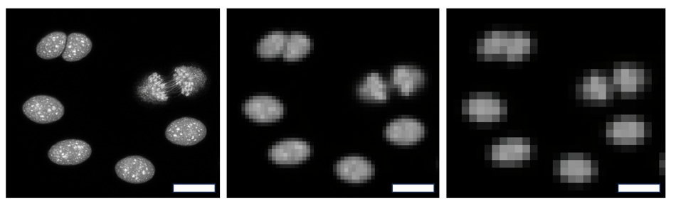
Figure
(Left) The pyramid of frustration. Imaging is a compromise where a user has to decide where the available photon budget goes. (Right) DNA acquired at different spatial sampling; scale bar 10 micrometer. Top Left: Intranuclear structures can be investigated. Middle: Intracellular structures are not visible but the number of nuclei could still be measured. Right: Nuclei start to blur so much rendering cell counting challenging. The lower panel is a zoom in.
A good way to explore what one can still see at different spatial samplings is to acquire an image with very fine sampling and then downsample it in a software. This can inform you how you would then acquire more images with optimal sampling of the microscope.
The two example images show the Z-maximal projection of several cells at a pixel-size of 35 nm (Zeiss Airy scan).
run("Close All")// Open the image//open("https://github.com/NEUBIAS/training-resources/raw/master/image_data/xy_16bit__DNA_sampling_35nm.tif")open("https://github.com/NEUBIAS/training-resources/raw/master/image_data/xy_16bit__MT_sampling_35nm.tif")rename("scaling_1");//Down scale with a factor of 2selectImage("scaling_1");run("Scale...","x=0.5 y=0.5 interpolation=Bilinear average create title=scaling_2.tif");//Down scale with a factor of 4selectImage("scaling_1");// Make sure you always start from the original imagefactor=4downsample=1/factorrun("Scale...","x="+downsample+" y="+downsample+" interpolation=Bilinear average create title=scaling_"+factor+".tif");//Down scale with a factor of 16selectImage("scaling_1");factor=16downsample=1/factorrun("Scale...","x="+downsample+" y="+downsample+" interpolation=Bilinear average create title=scaling_"+factor+".tif");
Assessment
Fill in the blanks
Over-sampling does not improve true optical resolution, but it increases _____, _____, and _____.