Getting started with the virtual microscope
A modern microscope is an imaging robot: its camera, stage, light sources and filters can all be controlled programmatically instead of through a graphical user interface. This enables custom automation, for example smart microscopy workflows in which the microscope analyzes its own images and decides what to do next.
Developing such workflows on a real instrument is slow and risky: every test costs instrument time and samples, and a bug can damage hardware. This module introduces a virtual microscope that lets you develop and test workflows without access to real hardware. Because the sample is simulated too, it can do things a real sample cannot: for example, time can run faster than in reality, so you do not have to wait for slow biology to respond and can run many more tests.
The virtual microscope builds on Micro-Manager and pymmcore-plus and implements exactly the same hardware interface as a real microscope running Micro-Manager. A script that works on the virtual microscope therefore runs on a real one after loading a different configuration file. In this module you install the virtual microscope, control it through its graphical user interface, and then do the same things from Python. Later modules reuse it, for example to learn how image feedback can automatically target specific regions with photostimulation.
Prerequisites
Before starting this lesson, you should be familiar with:
Basic Python (variables, functions, running a script)
Learning Objectives
After completing this lesson, learners should be able to:
Install the virtual microscope and launch its graphical user interface
Control the microscope programmatically: switch the objective, set the exposure, snap an image, set any device property
Explain how simulators (digital twins) help to develop and test smart microscopy workflows
Concept map
(napari + napari-micromanager)") --> C("pymmcore-plus") S("Python script") --> C C --> V("Virtual microscope") C -.-> R("Real microscope")
Figure
The software stack
The virtual microscope combines several tools whose names can be confusing at first, because they are often mentioned together. From the hardware up to what you see on screen:
- Micro-Manager is open-source microscope control software. Its most valuable part is a library of drivers (device adapters) for hundreds of cameras, stages, light sources and filter wheels, all behind one common interface. It also has its own graphical user interface, which this module does not use.
- pymmcore-plus gives Python access to that common interface. Your script holds a
coreobject and calls methods such ascore.snapImage(), and the core forwards each call to whichever devices are loaded. It also adds conveniences on top, such as notifications when a device changes and an acquisition engine for time-lapses and multi-position experiments. - napari is a Python image viewer, used across many image analysis workflows.
- napari-micromanager is a plugin that adds microscope controls to napari: snap, live view, channel and objective selection, exposure, stage control, acquisitions. Every control calls the same
coreobject that your scripts use. - The virtual microscope (the
virtual-microscope-teachingPython package) plugs simulated devices into pymmcore-plus in place of real hardware, together with a simulated sample in front of the simulated camera. Everything above it, pymmcore-plus, napari-micromanager and your scripts, works exactly as with a real microscope.
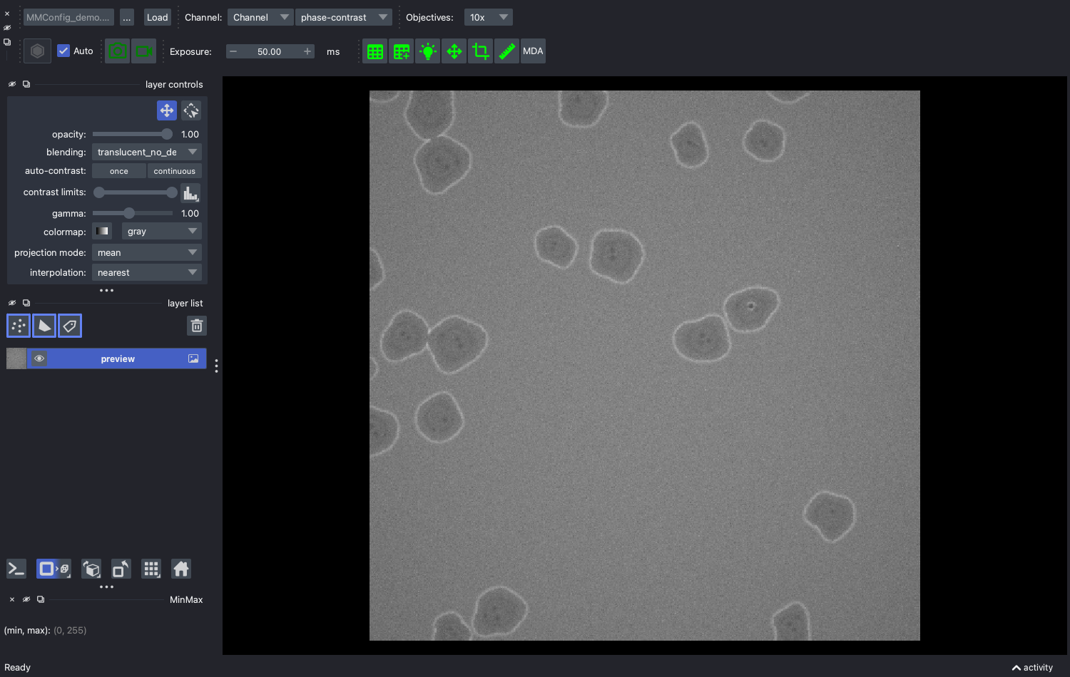
This is what the virtual microscope looks like in napari, with the napari-micromanager toolbars at the top:
Devices, properties and configurations
A few concepts from Micro-Manager appear in every script. They are the same on the virtual and on a real microscope.
Device. Each piece of hardware has a label, for example Camera, XYStage, Objective or LED.
Property. Every device has named properties that describe its state, for example the camera’s Exposure and Binning, or the LED’s Label (which light source is on). Each setting is therefore addressed by a triplet: device, property, value. core.setProperty("Camera", "Binning", 2) sets property Binning of device Camera to the value 2, and core.getProperty("Camera", "Binning") reads the current value back.
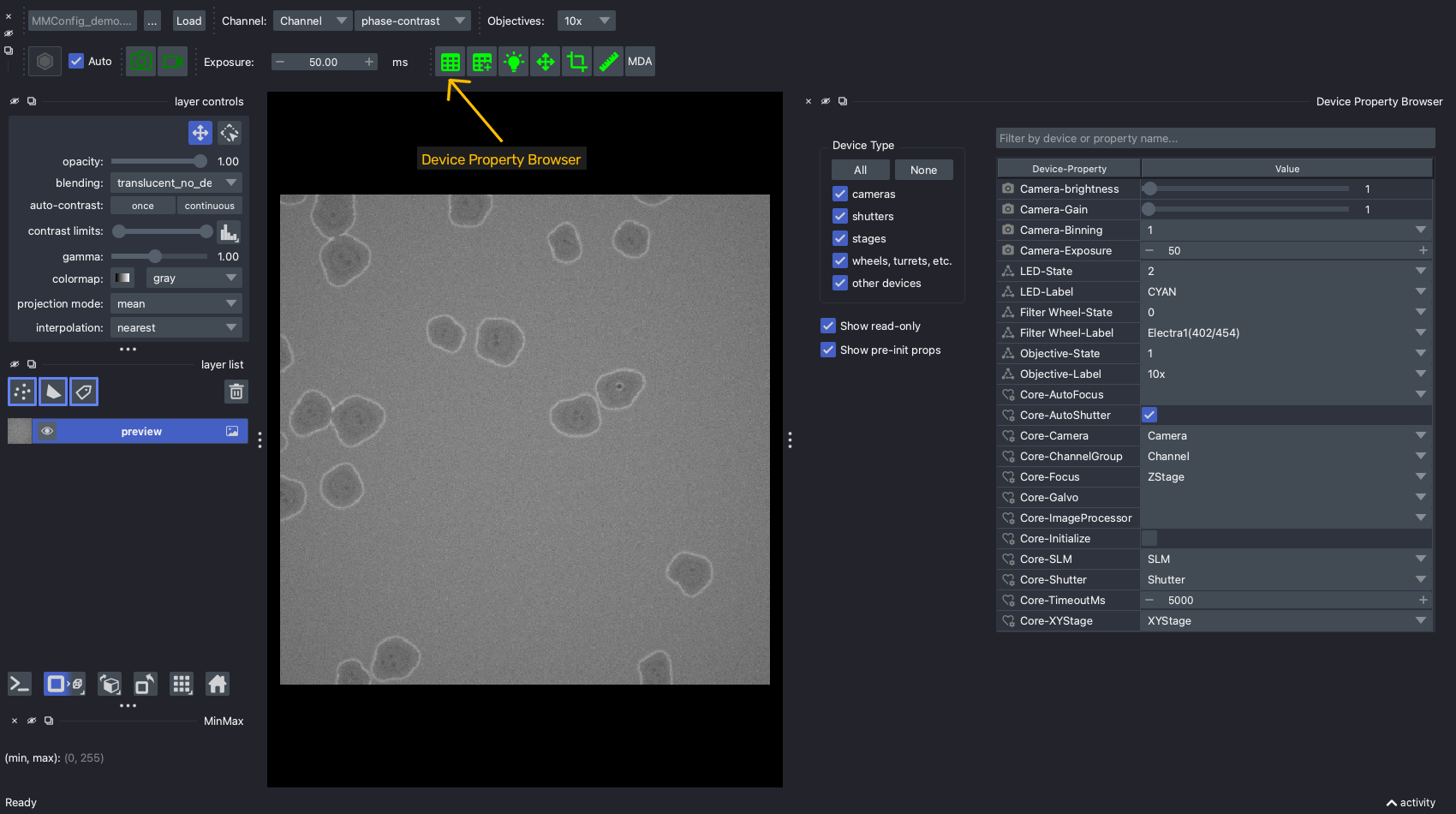
The Device Property Browser shows exactly these triplets, one per row: the Device-Property column names the device and the property (Camera-Binning), the Value column shows the current value. Use it to explore which devices your microscope has and which properties each one offers, and to change them by hand. Anything you can change there, a script can change too with core.setProperty. The browser opens from the first button of the napari-micromanager toolbar (arrow); here it is docked on the right:
Configuration group and preset. A named combination of property values that are usually changed together. In the Channel group, the preset miRFP sets the LED to the red light source and the filter wheel to the matching far-red emission filter. One line applies both:
core.setConfig("Channel", "miRFP")
It does exactly the same as the two separate property changes it stands for:
core.setProperty("LED", "Label", "RED")
core.setProperty("Filter Wheel", "Label", "miRFP670(642/670)")
After either version, core.getCurrentConfig("Channel") reports miRFP: a preset is nothing more than a name for a set of property values. The Channel dropdown in the GUI applies these presets, and you can watch the LED-Label and Filter Wheel-Label rows of the property browser change when you switch it.
Configuration file. A plain text file that tells the core which devices to load, which device plays which role (the camera, the focus drive, …), the configuration groups and presets, and the pixel size for each objective. Loading a different configuration file switches to a different microscope, for example from the virtual microscope to a real one. It is human-readable. An abridged excerpt of MMConfig_demo.cfg, the demo configuration that comes with Micro-Manager (its devices are Micro-Manager’s built-in demo devices, but the file looks the same for real hardware):
# Devices: label, device adapter (driver library), device in that library
Device,Camera,DemoCamera,DCam
Device,Emission,DemoCamera,DWheel
Device,Objective,DemoCamera,DObjective
Device,Z,DemoCamera,DStage
Device,XY,DemoCamera,DXYStage
...

# Roles: which device is the camera, the focus drive, ...
Property,Core,Camera,Camera
Property,Core,Focus,Z
...

# Labels: names for the positions of a filter wheel or turret
Label,Emission,0,Chroma-HQ620
Label,Emission,2,Chroma-HQ535
Label,Objective,1,Nikon 10X S Fluor
...

# Channel presets: group, preset, then device, property, value
ConfigGroup,Channel,DAPI,Emission,Label,Chroma-HQ620
ConfigGroup,Channel,FITC,Emission,Label,Chroma-HQ535
...

# Pixel size per objective, in um
ConfigPixelSize,Res10x,Objective,Label,Nikon 10X S Fluor
PixelSize_um,Res10x,1.0
Each preset line is again a device, property, value triplet, filed under a group and a preset name. On your own microscope, the configuration file is where to look up which devices it has and what its channel presets do. The virtual microscope’s file follows the same format; its device lines load the simulated Python devices instead of hardware drivers.
The GUI controls you will use and the calls a script makes to do the same:
| GUI control | What it does | Script equivalent |
|---|---|---|
| Snap (camera icon) | acquire one image into the preview layer |
core.snapImage(), then core.getImage() for the pixels |
| Live (film icon) | continuous acquisition | core.startContinuousSequenceAcquisition() |
| Channel dropdown | apply a channel preset | core.setConfig("Channel", "miRFP") |
| Objectives dropdown | switch the objective | core.setStateLabel("Objective", "40x") |
| Exposure box | exposure time in milliseconds | core.setExposure(100) |
| Stages Control (arrows icon) | move the stage | core.setXYPosition(x, y), focus: core.setPosition(z) |
| Device Property Browser (table icon) | set any property of any device | core.setProperty(device, property, value) |
The simulated sample
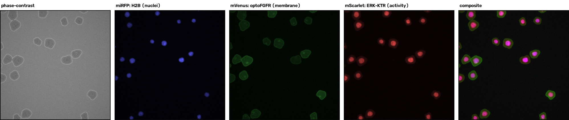
The virtual microscope can host different simulated samples. In this module and the modules that build on it, you will load the optogenetic sample (load_microscope("optogenetic")): live cells engineered with three fluorescent labels, plus a light-sensitive receptor whose role is explained in the follow-up module.
| Channel | Fluorophore labels | What you see |
|---|---|---|
phase-contrast |
(transmitted light) | all cells, label-free overview |
miRFP |
H2B, a histone: marks the nucleus | bright, well-separated nuclei on black |
mVenus |
optoFGFR, a membrane-bound receptor | the whole cell, slightly brighter at its edge, like a membrane stain |
mScarlet |
ERK-KTR, a kinase activity reporter | nucleus bright while the cell rests; the follow-up module puts this to work |
CyanStim |
(stimulation light path) | dark for now; used for photostimulation in the follow-up module |
Channels are named after the fluorophore, as they usually are on a real microscope, because the same fluorophore can label different proteins in different samples. The display colors in the composite are pseudo-colors chosen for contrast, not the emission colors.
The devices of the virtual microscope
| Device | What it simulates |
|---|---|
Camera |
a 512 x 512 pixel, 8-bit camera with exposure, gain and binning (1, 2 or 4); photon and read noise, a few hot pixels |
Objective |
a turret with 4x, 10x, 20x, 40x and 60x objectives. The image always stays 512 x 512 pixels; the pixel size and the field of view change, as on a real microscope |
XYStage |
moves the sample: two square wells side by side, with travel limits at the well edges |
ZStage |
the focus drive: moving away from the focal plane blurs the image |
LED |
the excitation light source, with several selectable wavelengths |
Filter Wheel |
the emission filters, one per fluorophore |
Shutter |
opens and closes the light path during acquisitions |
SLM |
a spatial light modulator (a DMD) that shapes the stimulation light into a pattern; used in the follow-up module |
What the simulation is, and is not
The simulated sample is a toy model: cells are soft shapes that crawl, protrude and bump into each other, and respond to light in a simplified way. It is designed to be easy to analyze, not to reproduce real cell biology, so do not draw biological conclusions from it. Nothing in the design prevents replacing it with a more realistic biophysical model; the virtual microscope can host different simulated samples, and the microscope side stays the same.
The microscope side reproduces what your control code interacts with: the devices, channels and presets, exposure and binning, objectives with their pixel sizes, optical blur and camera noise, and a stage with limits. It is not a perfect copy of real hardware either. The stage arrives at a new position instantly, where a real stage needs time to travel and settle. Filter wheels and light sources switch without delay, nothing drifts out of focus on its own, devices never time out or report errors, and the stimulation pattern lands exactly where it was meant to, where a real projector needs calibration. Treat a script that works on the simulator as ready for a first test on the real instrument, not as finished.
By default, the simulated sample evolves in real time while your code runs, like on a real microscope: your scripts wait with time.sleep as they would at the instrument, and the GUI shows every snap, channel switch and stimulation pattern live while an experiment runs. A simulator also offers two things a real sample never does. It can run faster than real time (speed=10: ten seconds of cell behavior per second of waiting), so slow biology such as migration can be tested in seconds. And in stepped mode (mode="stepped"), time advances only when your code says so (the advance() helper), so every run starts from exactly the same virtual sample and gives exactly the same result, on every machine. Automated tests and figure generation rely on that.
Activities
Explore the microscope through its GUI
You will operate the virtual microscope exactly like a real instrument, through the same graphical interface (napari-micromanager) that runs real Micro-Manager systems.
- Install the simulator and launch the microscope GUI with the optogenetic sample loaded (see the implementation tab for the exact commands)
- Explore the microscope interactively, like you would at a real instrument:
- Snap an image; start Live mode and watch the cells move
- Switch objectives (10x to 40x) and observe how the field of view shrinks while the image stays 512 x 512 pixels
- Step through the channels (phase-contrast, miRFP, mVenus, mScarlet) and compare what each label shows, as in the channel gallery above
- Change the exposure time and observe brightness and noise
- Move the stage to a different field of view, and to the edge of the well
- Open the Device Property Browser: find the properties that the Channel preset changes, and change the camera binning
Show activity for:
napari + Python
Installation
pip install "virtual-microscope-teaching[gui]"(Python 3.10 or newer. For the scripted part you can use any Python console or Jupyter. In Jupyter, run
%gui qtfirst.)Launch the microscope
The first argument of
load_microscopepicks the simulated sample; use"optogenetic"here and in the follow-up modules.from vmteach import load_microscope from vmteach.gui import launch_gui core, sim = load_microscope("optogenetic", n_cells=20, seed=0) viewer = launch_gui(core)napari opens with the napari-micromanager control toolbars, as in the screenshot in the module introduction.
Explore like at a real microscope
- Press Snap (camera icon): a
previewlayer appears- Press Live (film icon) for continuous acquisition: the cells ruffle and crawl
- Objectives dropdown: switch 10x to 40x and the field of view shrinks around the current stage position. 4x shows a large overview
- Channel dropdown: step through phase-contrast, miRFP, mVenus and mScarlet with Live running, and match what you see to the channel gallery. The fifth entry, CyanStim, is the stimulation light path used in the follow-up module; for now it shows a dark frame
- Exposure: increase and decrease it, and observe brightness and noise
- Stages Control (arrows icon in the toolbar): step the stage and watch new cells come into view. The two wells are 2048 um wide; at 4x, move toward the edge of a well until its wall and rounded corner appear in phase contrast
- Device Property Browser (table icon, the first in the toolbar): switch the Channel dropdown and watch the
LED-LabelandFilter Wheel-Labelrows change, since that is all a channel preset does. Then setCamera-Binningto 2: the image shrinks to 256 x 256 pixels and gets four times brighter, because each pixel now sums 2 x 2 sensor pixels. Lower the exposure to compensate, and set the binning back to 1
Drive the same microscope from code
Everything you just clicked is available as a function call on the same instrument. This equivalence is the foundation of microscope automation: a script is not “another program”, it is the same clicks issued by code.
- With the GUI still open, perform the same operations from Python and watch the GUI react: snap an image, switch the objective, switch the channel, change the exposure
- Read and change device properties from code, as in the Device Property Browser, and move the stage
- Retrieve a snapped image as a plain array and display it yourself
- Appreciate that GUI buttons and script commands issue the same control calls on the same microscope. Automation is scripted clicking, and on a real microscope the setup is identical: the GUI in front, your script behind, one shared core
Show activity for:
napari + Python
The GUI reacts to your code
Keep the napari window from the previous activity open. In the same Python session, run these one at a time and watch the GUI while each executes:
core.snapImage()                        # = pressing "Snap"; the preview layer updates
core.setStateLabel("Objective", "20x")  # = selecting "20x"; the dropdown follows
core.setConfig("Channel", "miRFP")      # = selecting "miRFP" in the Channel dropdown
core.setExposure(50.0)                  # = typing 50 in the Exposure box
core.snapImage()
The dropdowns now show 20x, miRFP and 50 ms: the GUI is a viewer onto the same
coreobject your script controls.Any property, and the stage
The Device Property Browser and your script read and write the same properties. With the browser open, run:
print(core.getProperty("LED", "Label"))         # the LED the miRFP preset selected
core.setProperty("Camera", "Binning", 2)        # watch the Binning row change
core.snapImage()
print(core.getImage().shape)                    # (256, 256)
core.setProperty("Camera", "Binning", 1)

print(core.getXYPosition())                     # stage position, um
core.setXYPosition(500.0, 0.0)                  # 500 um to the right: new cells
An image is just an array
Scripts do one thing the GUI cannot: hand the pixels to your own analysis code.
import matplotlib.pyplot as plt

core.snapImage()
img = core.getImage()               # a plain numpy array
print(img.shape, img.dtype, img.max())
plt.imshow(img, cmap="gray")
This is the bridge to everything that follows: once the image is an array, any image analysis can run on it, and its result can drive the next microscope command.
Reset for the next module
core.setXYPosition(0.0, 0.0)
core.setStateLabel("Objective", "10x")
core.setConfig("Channel", "phase-contrast")
core.setExposure(50.0)
Assessment
Scenario checks
- You have booked time on a real microscope anyway. Why develop and test your control script on the virtual microscope first? Name two things that are faster or safer to get wrong on the simulator, and one thing only the real instrument can tell you.
Solution
Faster or safer on the simulator, for example: debugging analysis and control logic (a crash costs seconds, not a sample or a damaged objective), trying out acquisition strategies, and developing without occupying the instrument. Another one is reproducibility: the virtual microscope can restart exactly the same virtual sample, so when you change your code and run again, any difference in the result comes from your code. On a real microscope every run starts from different cells in a different state, so two runs are never directly comparable. Only the real instrument can tell you how the real biology responds and how your specific hardware behaves (illumination, focus drift, sample health, actual signal levels).
- Think of your last session at the microscope. Which steps could a script do for you by replaying what you clicked in the GUI, and which steps needed you to be there?
Solution
Replayable steps are the ones that don’t require feedback: switching channels, setting exposures, moving through a list of stage positions, acquiring a time-lapse. Every GUI action is a call on the same core object scripts use, so these are straightforward to script. Steps that needed you were likely the ones where you looked at an image before deciding the next action: finding a good field of view, choosing which cells to image or stimulate, refocusing when the sample drifted. Automating those needs image analysis in the loop, the microscope reacting to its own images. That is feedback control, the topic of the follow-up modules.
- Your control script runs perfectly on the virtual microscope. On the real instrument it stops at the line that switches to a channel that does not exist there. Where would you look first, and what other differences should you expect between the two?
Solution
First in the configuration: channel presets are defined per instrument in its configuration file, so the real system needs a preset with that name, or the script must use the real system’s name. Both microscopes expose the same interface, so many differences live in the configuration rather than the control logic. Do not expect it to end there, though: controlling real hardware is still difficult, and devices differ in subtle ways, for example cameras with a different bit depth or timing, stages that take time to travel and settle between positions, or light sources that need time to warm up. When you find that your system behaves differently in a way that matters for your script, consider modelling that behaviour in the simulator, so that the next test catches it before the real experiment does.
Discuss with your neighbour
- What could a simulated microscope never tell you about your real experiment?
- Which quirk of your own microscope would you add to the simulator first, and how would it change the way you write your scripts?
- Think of the last experiment that went wrong at the microscope. Would any part of that failure have shown up while testing on a simulated instrument? Which part could only have failed on the real one?
Follow-up material
Recommended follow-up modules:
Learn more: