Batch processing

Prerequisites

Before starting this lesson, you should be familiar with:

• Strings and paths

• For loops

Learning Objectives

After completing this lesson, learners should be able to:

• Automatically process a number of images

Motivation

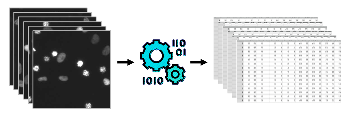
Scientific discovery is based on reproducibility. Thus, it is very common to apply the same analysis workflow to a number of images, possibly comprising different biological conditions. To achieve this, it is very important to know how to efficiently “batch process” many images.

Concept map

Figure

Activities

Batch analysis of nuclear shapes

• In a previous module there is a workflow to measure the shapes of nuclei in one image
• Adapt this workflow for automated batch analysis of many images

• Start by building the skeleton of the workflow without filling in the functionality;

  Note that the code below runs fine, but does not produce any results:

def analyse(image_path, output_folder):
    print("Analyzing:", image_path)
    
for image_path in image_paths:
    analyse(image_path, output_dir)

• Make sure the loop with the (almost) empty analyse function runs without error before filling in the image analysis steps

ImageJ SciJava Macro

/**

• 2D Nuclei area measurement
• Requirements:
• • Update site: IJPB-Plugins (MorpholibJ) */

// Scijava script parameters // Use the [ Batch ] button in the Fiji script editor to automatically analyse multiple files #@ File (label=”Input image”) inputImageFile #@ File (label=”Output directory”, style=”directory”) outputDir

// Processing parameters threshold = 25;

// Clean up and avoid popping up of image windows during run run(“Close All”); run(“Clear Results); setBatchMode(true);

// init options run(“Options…”, “iterations=1 count=1 black do=Nothing”);

// open and process // open(inputImageFile);

// extract image name to create output file names (s.b.) imageName = File.getNameWithoutExtension(inputImageFile);

// segment setThreshold(threshold, 65535); run(“Convert to Mask”); run(“Connected Components Labeling”, “connectivity=4 type=[8 bits]”); run(“glasbey_on_dark”); // save segmentation saveAs(“Tiff”, outputDir + File.separator + imageName + “_labels.tif”); // measure run(“Analyze Regions”, “area”); // save measurements saveAs(“Results”, outputDir + File.separator + imageName + “.txt”);

run(“Close” ); // close results table

skimage python

# %% 
# Batch analysis of 2D nuclei shape measurements

# %%
# Import python modules
from OpenIJTIFF import open_ij_tiff, save_ij_tiff
from skimage.measure import label, regionprops_table
from skimage.filters import threshold_otsu
import pandas as pd
import pathlib
from pathlib import Path
from napari import Viewer

# %%
# Create a function that analyses one image
# Below, this function will be called several times, for all images
def analyse(image_path, output_folder):

    # This prints which image is currently analysed
    print("Analyzing:", image_path)

    image, axes, scales, units = open_ij_tiff(image_path)

    # Binarize the image using auto-thresholding
    threshold = threshold_otsu(image)
    print("Threshold:", threshold)
    binary_image = image > threshold

    # Perform connected components analysis (i.e create labels)
    # Note that label returns 32 bit data which save_ij_tif below can't handle.
    # We can safely convert to 16 bit as we know that we don't have too many objects
    label_image = label(binary_image).astype('uint16')

    # Measure calibrated (scaled) nuclei shapes
    df = pd.DataFrame(regionprops_table(
        label_image,
        properties={'label', 'area'},
        spacing=scales))

    # Round all measurements to 2 decimal places.
    # This increases the readability a lot,
    # but depending on your scientific question,
    # you may not want to round that much!
    df = df.round(2)

    # Save the results to disk

    # Convert the image_path String to a Path,
    # which is more convenient to create the output files
    image_path = pathlib.Path(image_path)

    # Save the labels
    label_image_path = output_folder / f"{image_path.stem}_labels.tif"
    save_ij_tiff(label_image_path, label_image, axes, scales, units)

    # Save the measurements table
    # to a tab delimited text file (sep='\t')
    # without row numbers (index=False)
    table_path = output_folder / f"{image_path.stem}_measurements.csv"
    df.to_csv(table_path, sep='\t', index=False)
    

# %%
# Assign an output folder 
# Note: This uses your current working directory; you may want to change this to another folder on your computer
output_dir = Path.cwd()

# %%
# Create a list of the paths to all data
image_paths = ["https://github.com/NEUBIAS/training-resources/raw/master/image_data/xy_8bit__mitocheck_incenp_t1.tif", 
               "https://github.com/NEUBIAS/training-resources/raw/master/image_data/xy_8bit__mitocheck_incenp_t70.tif"]

for image_path in image_paths:
    analyse(image_path, output_dir)

# %%
# Plot the first output image to check if the pipeline worked
image1, *_ = open_ij_tiff(image_paths[0])
labels1, *_ = open_ij_tiff('xy_8bit__mitocheck_incenp_t1_labels.tif')

viewer = Viewer()
viewer.add_image(image1)
viewer.add_labels(labels1)

Assessment

Fill in the blanks

1. If you have thousands of images to process you should consider using a ___ .
2. Batch processing refers to __ processing many data sets.

Solution

1. computer cluster (HPC)
2. automatically

Explanations

Follow-up material

Recommended follow-up modules:

Learn more:

• Batch processing in ImageJ