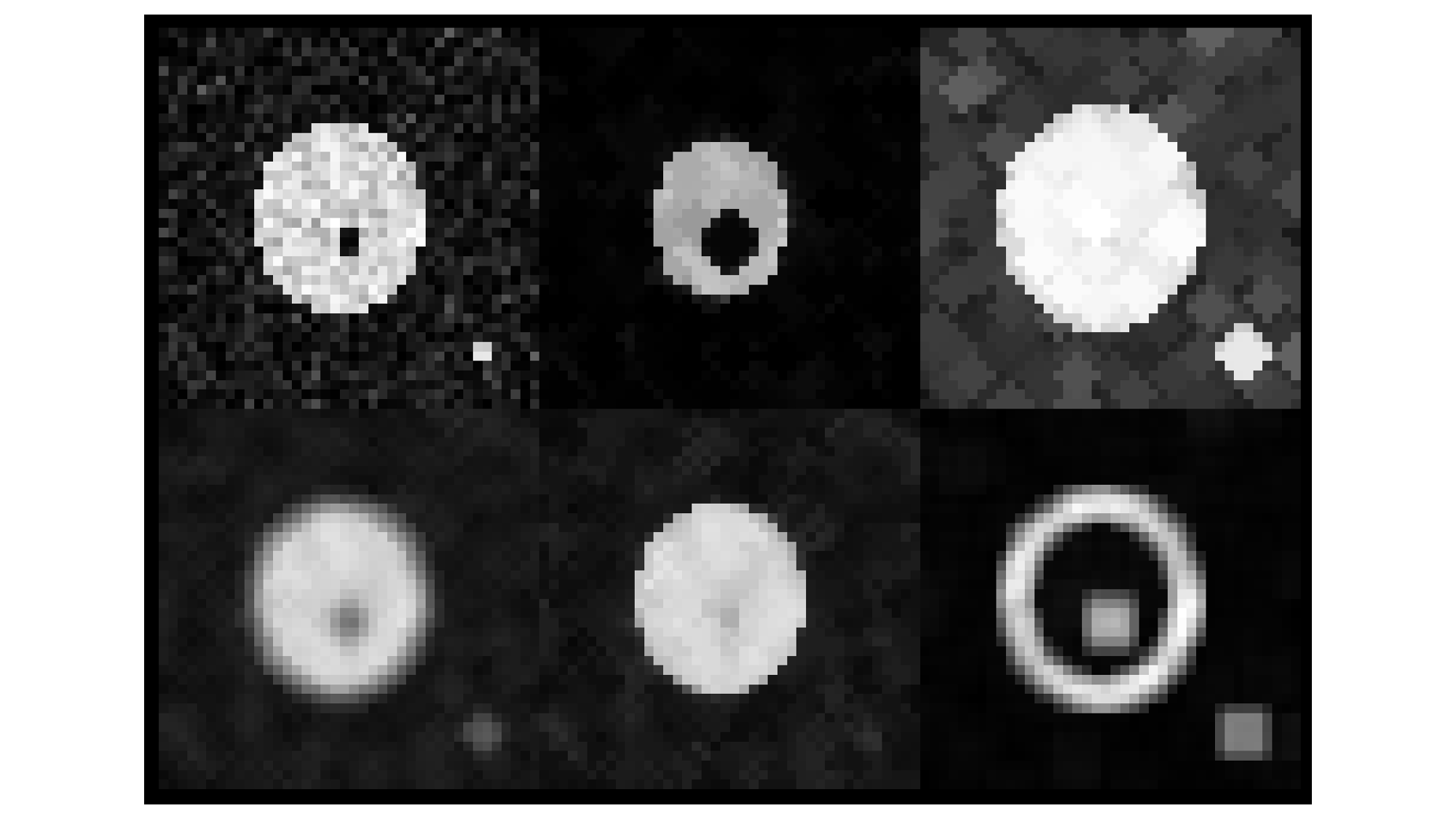
Shows the effect of a radius 2 disk shaped kernel statistical filter on an image. Top left: Input; Top middle: Minimum; Top right: Maximum; Bottom left: Mean; Bottom middle: Median; Bottom right: Variance.
Explore the effect of the median filter on various example images. Explore how changing the size (structural element) of the filter affects the result.
Observe how the median filter behaves for binary images.
Show activity for:
ImageJ Macro
run("Close All");//File > Open...open("https://github.com/NEUBIAS/training-resources/raw/master/image_data/xy_8bit__two_noisy_squares_different_size.tif");// Image > Duplicate...run("Duplicate...","title=Median_1");// Image > Duplicate...run("Duplicate...","title=Median_2");// Image > Duplicate...run("Duplicate...","title=Median_5");selectWindow("Median_1");// Process › Filters › Median...run("Median...","radius=1");selectWindow("Median_2");// Process › Filters › Median...run("Median...","radius=2");selectWindow("Median_5");// Process › Filters › Median...run("Median...","radius=5");run("Tile")
skimage napari
# %%
# Median filtering
# %%
# import modules
importnapariimportnumpyasnpfromskimageimportfiltersfromskimage.filtersimportrankfromskimage.morphologyimportdisk# Structuring element
fromOpenIJTIFFimportopen_ij_tiff# %%
# Instantiate the napari viewer
viewer=napari.Viewer()# %%
# Read and view the image
image,*_=open_ij_tiff('https://github.com/NEUBIAS/training-resources/raw/master/image_data/xy_8bit__two_noisy_squares_different_size.tif')viewer.add_image(image)# %%
# Compare small median and mean filter
# - Appreciate that the median filter better preserves the edges
median_1=filters.median(image,disk(1))viewer.add_image(median_1)mean_1=rank.mean(image,disk(1))viewer.add_image(mean_1)# %%
# Compare a larger median and mean filter
# - Appreciate that a median filter eliminates the small square entirely
median_3=filters.median(image,disk(3))viewer.add_image(median_3)mean_3=rank.mean(image,disk(3))viewer.add_image(mean_3)########### New image: nucleare speckles #############
# %%
# Clear the napari viewer
viewer.layers.clear()# %%
# Load image
image,*_=open_ij_tiff('https://github.com/NEUBIAS/training-resources/raw/master/image_data/xy_8bit__PCNA.tif')# %%
# View the image and find the radius of the intra-nuclear speckles
viewer.add_image(image)# %%
# Remove small intra-nuclear structures
# - Appreciate that a median filter removes the intra-nuclear speckles while keeping the nuclear shape intact
# - This can be helpful in many ways, e.g. some deep learning nuclear segmentation tools get confused by intra-nuclear speckles
# - Another application is to subtract the filtered image from the original image to only have the speckles; this will be used in the
# "local background subtraction" training module
image_without_speckles=filters.median(image,disk(radius=15))viewer.add_image(image_without_speckles)# %%
# Close the viewer (CI test requires this)
viewer.close()
Once the upload is finished, click the Close button at the bottom of the upload window
The uploaded images will be available in your Galaxy history on the right panel.
Apply Median Filter
In the Tools panel, search Filter 2D image, and click Filter 2D image with scikit-image from the search results
In Galaxy main window,apply the followings
Filter type: Median
Radius/Sigma: Explore different values, such as 1,2 or 5
Source file: click the second button to activate Multiple datasets. Select images from the dropdown list.
Click Run Tool
Depending on the number of input images, you will see the corresponding number of outputs in the History panel on the right. Wait for them to turn green and download the resulting images.
run("Close All");// File > Open...open("https://github.com/NEUBIAS/training-resources/raw/master/image_data/xy_8bit__statistical_filter_test_input.tif");zoom();// Manual activity:// Choose one interesting 5x5 region// in the image and manually compute// the below statistical filters.// Note down the resulting numbers and later check// whether they agree with the below// automated analysis.// Image > Duplicate...run("Duplicate...","title=Minimum");zoom();run("Duplicate...","title=Maximum");zoom();run("Duplicate...","title=Mean");zoom();run("Duplicate...","title=Median");zoom();run("Duplicate...","title=Variance");zoom();// Apply Minimum filterselectWindow("Minimum");// Process › Filters › Minimum...run("Minimum...","radius=2");// Apply Maximum filterselectWindow("Maximum");// Process › Filters › Maximum...run("Maximum...","radius=2");// Apply Mean filterselectWindow("Mean");run("32-bit");// Results of mean filter are generally not 8=bit// Process › Filters › Mean...run("Mean...","radius=2");// Apply Median filterselectWindow("Median");// Process › Filters › Median...run("Median...","radius=2");// Apply Variance filterselectWindow("Variance");run("32-bit");// Results of variance filter are generally not 8=bit// Process › Filters › Variance...run("Variance...","radius=2");// Arrange windows in a tiled layoutrun("Tile");// Learning opportunities:// - Check the result of a variance filter without converting the image to 32-bit floatfunctionzoom(){run("In [+]");run("In [+]");run("In [+]");run("In [+]");}
skimage napari
# %%
# Statistical filtering
# %%
# Import modules
importnapariimportnumpyasnpfromskimageimportiofromskimage.filtersimportrankfromskimage.morphologyimportdisk# Structuring element
fromskimageimportimg_as_float,img_as_ubytefromOpenIJTIFFimportopen_ij_tiff# %%
# Instantiate the napari viewer
viewer=napari.Viewer()# %%
# Read and view the image
image,*_=open_ij_tiff('https://github.com/NEUBIAS/training-resources/raw/master/image_data/xy_8bit__statistical_filter_test_input.tif')viewer.add_image(image,name="Original")# %%
# Apply Minimum filter
# - Removes bright details smaller than the structuring element
minimum_filtered=rank.minimum(image,disk(2))viewer.add_image(minimum_filtered,name="Minimum (r=2)")# %%
# Apply Maximum filter
# - Removes dark details smaller than the structuring element
maximum_filtered=rank.maximum(image,disk(2))viewer.add_image(maximum_filtered,name="Maximum (r=2)")# %%
# Apply Mean filter
# - Smooths the image by averaging pixels within the structuring element
mean_filtered=rank.mean(image,disk(2))viewer.add_image(mean_filtered,name="Mean (r=2)")# %%
# Apply Median filter
# - Removes noise while preserving edges
median_filtered=rank.median(image,disk(2))viewer.add_image(median_filtered,name="Median (r=2)")
Apply a variance filter [ Process > Filter > Variance… ] to segment the cell regions from the background
Hints:
Convert image to float or 16 bit, because the filter may yield high values [ Image > Type > 32-bit ]
What filter radius and threshold yield a good segmentation?
Solution
[ Image › Rename…]
Title = input
[ Image › Duplicate… ]
Title = variance_5
[ Image > Type > 32-bit ]
In variance calculation, pixel values can exceed 255 which is the maximum value that can be achieved in current bit depth (unsigned 8-bit) of input image.
[ Process › Filters › Variance… ]
Radius = 15 pixels
[ Image › Adjust › Threshold… ]
([x] Dark Background)
Lower threshold level = 90 (1.5 for second example)
Higher threshold level = 1e30
Press Set
Press Apply
Press Convert to Mask
ImageJ Macro
// File > Close Allrun("Close All");// File > Openopen("https://github.com/NEUBIAS/training-resources/raw/master/image_data/xy_8bit__em_mitochondria_er.tif");// Image › Duplicate...run("Duplicate...","title=variance_5");// Image > Type > 16-bit (since in variance calculation values can exceed 255 which is current bit depth of input image)run("16-bit");// Process › Filters › Variance...run("Variance...","radius=5");// Image › Duplicate…run("Duplicate...","title=binary");// Image › Adjust › Threshold... ([x] Dark Background)setAutoThreshold("Default dark");//Press `Set` button (example upper and lower threshold values are (113, 255))setThreshold(90,1e30);// Press `Apply` buttonrun("Convert to Mask");// Image › Lookup Tables › InvertLUT... (if highest values are darker and lowest brighter)run("Invert LUT");// Window > Tilerun("Tile");
skimage napari
# %%
# Statistical filtering
# %%
# Import modules
importnapariimportnumpyasnpfromskimageimportiofromskimage.filtersimportrankfromskimage.morphologyimportdiskfromskimageimportimg_as_float,img_as_ubytefromscipy.ndimageimportgeneric_filterfromOpenIJTIFFimportopen_ij_tiff# %%
# Instantiate the napari viewer
viewer=napari.Viewer()# %%
# Read and view the image
image,*_=open_ij_tiff('https://github.com/NEUBIAS/training-resources/raw/master/image_data/xy_8bit__em_mitochondria_er.tif')viewer.add_image(image,name="Original")# %%
# Apply Variance filter
# - Highlights areas with high intensity variation
variance_filtered=generic_filter(image.astype(float),function=np.var,size=5)viewer.add_image(variance_filtered,name="Variance (r=5)")viewer.grid.enabled=True# %%
# Learning opportunity:
# - Check the output of the variance filter without converting to float datatype
# - Explore how changing the size of the filter kernels affects the output
# - Apply a threshold
binary=variance_filtered>90viewer.add_image(binary,name="binary")# %%
# Close the viewer (CI test requires this)
viewer.close()
Assessment
Answer the questions
What is the primary purpose of applying a median filter to an image?
How does a local maximum filter differ from a local minimum filter in terms of the output pixel values?
Why might variance filtering be particularly useful in label-free microscopy?
Solution
To reduce noise in an image while preserving edges.
A local maximum filter replaces each pixel with the maximum value in its neighborhood, while a local minimum filter replaces it with the minimum value.
Variance filtering highlights regions with high variability, which can help detect structures in label-free microscopy such as transmission light microscopy or electron microscopy.