Our eyes are extremely good in distinguishing forms and patterns and this has proven to be a powerful tool for characterizing different cell-types, functions, phenotypes, and more. In image processing, we use shape measurements (e.g. area, volume, elongation, …) for an automated and objective characterization of forms. Consequently, one can address scientific questions or filter objects that should be used for further processing.
Prerequisites
Before starting this lesson, you should be familiar with:
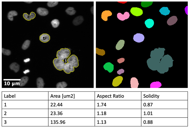
Left: Fluorescence microscopy of nuclei showing various shapes with three nuclei manually delineated. Right: Label mask image of all nuclei. Bottom: Table with some shape measurements of the manually delineated nuclei.
#%%
# Measure shapes in 2D
#%%
fromOpenIJTIFFimportopen_ij_tiffimportnapari#%%
# Open a label image with a few objects
labels,axes,scales,units=open_ij_tiff("https://github.com/NEUBIAS/training-resources/raw/master/image_data/xy_8bit_labels__four_objects.tif")#%%
# Show the label image in napari
viewer=napari.Viewer()viewer.add_labels(labels)#%%
# Perform shape measurements and discuss their meanings
# See: https://scikit-image.org/docs/stable/api/skimage.measure.html#skimage.measure.regionprops
fromskimage.measureimportregionprops_tableimportpandasaspdproperties=['label','area','perimeter','eccentricity','major_axis_length','minor_axis_length','solidity']table=regionprops_table(labels,properties=properties)print(type(table))df=pd.DataFrame(table)print(type(df))print(df)#%%
# Perform scaled (calibrated) shape measurement
# - Observe which shape measurements are changing due to the scaling
df=pd.DataFrame(regionprops_table(labels,properties=properties,spacing=scales))print(df)#%%
# Find the object with the biggest area
print(df['area'].max())print(df['area'].idxmax())print(df['label'][0])# i.e. df['label'][df['area'].idxmax()]
#%%
# Save the table as a CSV
df.to_csv('shape_measurements.csv',sep='\t',index=False)# %%
# Close the viewer (CI test requires this)
viewer.close()
Measure object shapes and find the label index of the nucleus with the largest perimeter
Change the pixel size to 0.5 um and repeat the measurements. Why do some parameters change while others don’t?
(Optional) Create an image where each object is coloured according to the measured circularity
Solution
[Plugins > MorphoLibJ > Analyze > Analyze Regions] the upper right nuclei.
Some features are the ratio of dimensional features and so are independent of the spatial calibration.
[Plugins > MorphoLibJ > Label Regions > Assign Measure to Label].
skimage napari
#%%
# Practice measure shape
#%%
fromOpenIJTIFFimportopen_ij_tiffimportmatplotlib.pyplotaspltimportnapariimportnumpyasnpfromskimage.measureimportregionprops,regionprops_table#%%
# Open image [xy_16bit_labels__nuclei.tif](https://github.com/NEUBIAS/training-resources/raw/master/image_data/xy_16bit_labels__nuclei.tif)
image,axes_image,scales_image,units_image=open_ij_tiff("https://github.com/NEUBIAS/training-resources/raw/master/image_data/xy_16bit_labels__nuclei.tif")#%%
viewer=napari.Viewer()label_layer=viewer.add_labels(image,name="eccentricity")#%%
# Measure object shapes
shape_measurements=regionprops(image)# Print perimeter and eccentricity of each label
forregioninshape_measurements:print(region.label,region.perimeter,region.eccentricity)#%%
# Optional: find the label index of the nucleus with the largest perimeter
perimeters=[region.perimeterforregioninshape_measurements]labels=[region.labelforregioninshape_measurements]idx_max_perimeter=np.argmax(perimeters)label_max_perimeter=labels[idx_max_perimeter]print('Largest perimeter:',np.max(perimeters))print('Label with largest perimeter:',label_max_perimeter)#%%
# Change the pixel size to 0.5 um and repeat the measurements. Why do some parameters change while others don't?
shape_measurements_scaled=regionprops(image,spacing=scales_image)forregioninshape_measurements_scaled:print(region.label,region.perimeter,region.eccentricity)#%%
# Optional: Create an image where each object is colored according to the measured circularity
shape_measurements_table=regionprops_table(image,properties=("label","eccentricity"))#%%
colors=plt.cm.viridis(shape_measurements_table["eccentricity"])label_layer.color_mode="direct"label_layer.color=dict(zip(shape_measurements_table["label"],colors))# %%
# Close the viewer (CI test requires this)
viewer.close()plt.close('all')
Assessment
True or false? Discuss with your neighbour
Circularity is independent of image calibration.
Area is independent of image calibration.
Perimeter can strongly depend on spatial sampling.
Volume can strongly depend on spatial sampling.
Drawing test images to check how certain shape parameters behave is a good idea.
Solution
Circularity is independent of image calibration True
Area is independent of image calibration. False
Perimeter can strongly depend on spatial sampling. True
Volume can strongly depend on spatial sampling. True
Drawing test images to check how certain shape parameters behave is a good idea. True