We use distance transform to quantify how a structure of interest is away from object boundaries or other structures. The distance transform is also use to characterize the morphology of an object in 2D and 3D, find its center, dimensions, etc.. Finally distance transform can be used as a pre-processing step to improve the segmentation results and split touching objects.
Prerequisites
Before starting this lesson, you should be familiar with:
After completing this lesson, learners should be able to:
Understand how to use distance transform to quantify morphology of objects
Understand how to use distance transform to quantify distance between objects
Understand approximate nature of distance transform
Concept map
graph TD
B[Binary image] --> DT(Distance transform)
DT --> D["Distance map image"]
D -- contains --- DN("Distances to nearest background pixel")
D -- is --- A("Approximation of euclidian distance")
DT -- has --- VI("Various implementations")
Figure
Upper panel - Binary image and the corresponding distance map. The distance map has three local maxima, which are very useful for object splitting and defining object centers. Lower panel - Inverted binary image and corresponding distance map, which is useful to compute distances to closest objects.
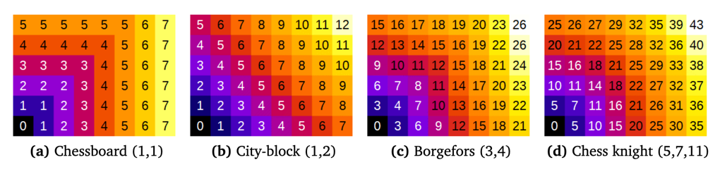
Chamfer distance (modified from MorpholibJ Manual)
Several methods (metrics) exist for computing distance maps. The MorphoLibJ library implements
distance transforms based on chamfer distances. Chamfer distances approximate Euclidean
distances with integer weights, and are simpler to compute than exact Euclidean distance
(Borgefors, 1984, 1986). As chamfer weights are only an approximation of the real Euclidean
distance, some differences are expected compared to the actual Euclidean distance map.
Several choices for chamfer weights are illustrated in above Figure (showing the not normalized distance).
The “Chessboard” distance, also named Chebyshev distance, gives the number of moves that an imaginary Chess-king needs to reach a specific pixel. A king can move one pixel in each direction.
The “City-block” distance, also named Manhattan metric, weights diagonal moves differently.
The “Borgefors” weights were claimed to be best approximation when considering the 3-by-3 neighborhood.
The “Chess knight” distance also takes into account the pixels located at a distance from
(±1, ±2) in any direction. It is usually the best choice, as it considers a larger neighborhood.
To remove the scaling effect due to weights > 1, it is necessary to perform a normalization step. In MorphoLibJ this is performed by dividing the resulting image by the first weight (option Normalize weights).
Perform an intensity gating on the distance map, e.g. by thresholding, to create a mask with all pixels of a certain distance, e.g. between 100-120, to the reference object.
/*
* Requirements:
* - MorpholibJ, Update site: IJPB-Plugins
*
**/// Distance measurementsrun("Close All");open("https://github.com/NEUBIAS/training-resources/raw/master/image_data/xy_8bit_labels__dist_trafo_b.tif");rename("labels");// Make invert mask of first labelrun("Duplicate...","title=binary");run("Manual Threshold...","min=1 max=1");run("Convert to Mask");run("Invert");// Compute distance transform run("Chamfer Distance Map","distances=[Chessknight (5,7,11)] output=[32 bits] normalize");rename("dist");run("Intensity Measurements 2D/3D","input=dist labels=labels mean max min");
Region selection, ImageJ Macro MorpholibJ
/*
* Requirements:
* - MorpholibJ, Update site: IJPB-Plugins
*
**/// Region selection by Distance gatingopen("https://github.com/NEUBIAS/training-resources/raw/master/image_data/xy_8bit_binary__single_object.tif");run("Invert");run("Chamfer Distance Map","distances=[Chessknight (5,7,11)] output=[16 bits] normalize");run("Manual Threshold...","min=100 max=120");run("Convert to Mask");
Python Napari
# Distance transform with skimage using napari as a viewer
importimageio.v3asimageiofromOpenIJTIFFimportopen_ij_tiffimportnaparifromscipyimportndimageif'viewer'notinglobals():viewer=napari.Viewer()image,*_=open_ij_tiff('https://github.com/NEUBIAS/training-resources''/raw/master/image_data/xy_8bit_labels__four_objects.tif')print(image.dtype)distance_map=ndimage.distance_transform_edt(image)print(distance_map.dtype)viewer.add_image(image)viewer.add_image(distance_map)# %%
# Close the viewer (CI test requires this)
viewer.close()
Exercises
Measure distance to center of cell
We would like to measure the distance within a binary mask to a specific point in the cell. This is called Geodesic distance.
Compute the geodesic distance map of the binary image with respect to a reference point close to the soma of the cell (approx x_pixel = 88, y_pixel = 74)
Measure thickness of glial branches
The goal is to combine skeletonization and distance map computation to measure skeleton branch length and thickness. For this exercise you need the binary image xy_8bit_binary__glialcell.tif and the skeletonized and normalized version xy_8bit_binary__glialcell_skeleton.tif
Use the image calculator function [ Process › Image Calculator…] to multiply the skeleton image by the distance map:
Image1: Skeleton
Operation: Multiply
Image2: Distance map
‘create new window’
‘32-bit float result’
[ Image › Lookup Tables › Fire]
Obtain branch information by analyzing the skeleton: [Analyze › Skeleton › Analyze Skeleton (2D/3D)]
‘Prune ends’
‘Calculate largest shortest path’
‘Show detailed info’
‘Display labeled skeletons’.
In the ‘Branch information’ table, you can find information on branch length, as well as average intensity. Since the distance map tells you the distance a pixel is away from the boundary, you can estimate the average branch thickness by multiplying this value by 2.
Assessment
Discuss with your neighbor
Knowing the image calibration, how could we convert a 2D distance map to physical values?
Knowing the image calibration, how could we convert a 3D distance map to physical values? Is it important if the image is isotropic sampled or not?