Morphological filters (MFs) are used to clean up segmentation masks and achieve a change in morphology and/or size of the objects. For example, MFs are used to remove wrongly assigned foreground pixels, separate touching objects, or identify objects boundaries.
Prerequisites
Before starting this lesson, you should be familiar with:
After completing this lesson, learners should be able to:
Understand how to design morphological filters using rank filters
Execute morphological filters on binary or label images and understand the output
Concept map
graph TD
subgraph opening
erode("Erode (min)") --> dilate("Dilate (max)")
end
subgraph closing
dilate2("Dilate (max)") --> erode2("Erode (min)")
end
subgraph rank operations
any("...")
end
BI("Binary/label image") --> SE("structuring element")
SE .-> erode
SE .-> dilate2
SE .-> any
dilate .-> BIM
erode2 .-> BIM
any .-> BIM("Modified binary/label image")
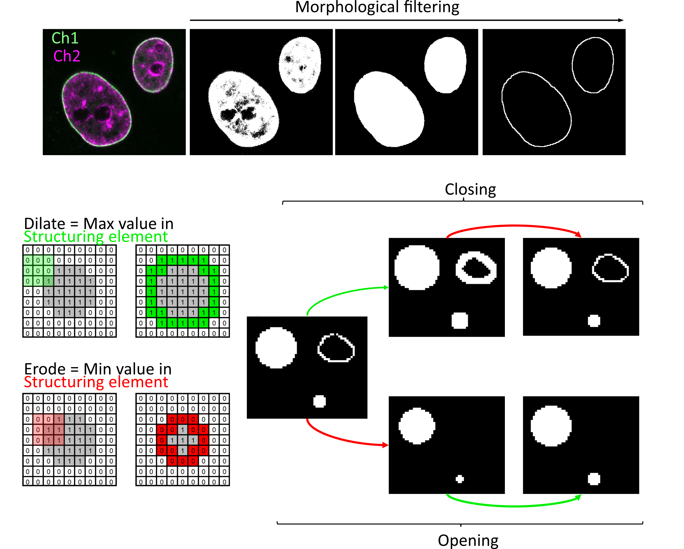
Figure
Upper row - Example of a workflow using morphological filters to improve the segmentation and compute the edge of the nuclei for further intensity measurements if necessary measurements have to be made on the periphery. Image on top left is a 2 channel intensity image (where channel 1 shows nuclear membrane and channel 2 shows dna staining). Lower row - Image level description of dilation and erosion operation using a 3x3 structuring element (left side). Morphological filters applied in series, e.g. opening (i.e. erosion followed by dilation) and closing (i.e. dilation followed by erosion), can achieve very useful results (right side). Red and green arrows show erosion and dilation respectively
Rank filters
In the region defined by the structuring element, pixel elements are ranked/sorted according to their values. The pixel in the filtered image is replaced with the corresponding sorted pixel (smallest = min, greatest = max, median ). See also Median filter. Morphological filters corresponds to one or several rank filters applied to an image.
Morphological filters on binary images
A typical application of these filters is to refine segmentation results. A max-filter is called dilation whereas a min-filter is called erosion. Often rank filters are applied in a sequence. We refer to a closing operation as a max-filter followed by a min-filter of the same size. An opening operation is the inverse, a min-filter followed by a max-filter.
Opening operations will:
Remove small/thin objects which extent is below the size of the structuring element
Smooth border of an object
Closing operations:
Fill small holes below the size of the structuring element
Can connect gaps
Image subtraction using eroded/dilated images allows to identify the boundary of objects and is referred to morphological gradients:
Internal gradient: original - eroded
External gradient: dilated - original
(Symmetric) gradient: dilated - eroded
Fill holes operation is a slightly more complex morphological operation. It is used to identify background pixels surrounded by foreground pixels and change their value to foreground. Algorithmically there are several ways to achieve this.
Morphological filters on label images
Morphological filters work also on label images. If the objects are not touching this will achieve the expected result for each label. However, when objects touch each other, operations such as dilations can lead to unwanted results.
Morphological filters on grey level images
Min and max operations can be applied to grey level images. Applications are for example contrast enhancement, edge detection, feature description, or pre-processing for segmentation.
Appreciate how structures grow and shrink or even disappear depending on the size of the structuring element
Show activity for:
ImageJ Macro
run("Close All");//Make sure black background in Process > Binary > Options is set to truesetOption("black background",true);open("https://github.com/NEUBIAS/training-resources/raw/master/image_data/xy_8bit_binary__three_spots_different_size.tif");// Image > Renamerename("binary");run("Set... ","zoom=400 x=29 y=25");// Erosion, use default binary IJ binary operations// It is a radius 1 squared SE, i.e. 3x3 SE// Image > Duplicate, name it erodedrun("Duplicate...","title=eroded");//Process > Binary > Eroderun("Erode");run("Set... ","zoom=400 x=29 y=25");// Apply second erosion will remove small dot// Image > Duplicate, name it eroded_twicerun("Duplicate...","title=eroded_twice");// Process > Binary > Eroderun("Erode");run("Set... ","zoom=400 x=29 y=25");// Use MorpholibJ and a radius 2, i.e. 5x5 squared structuring element// This corresponds to 2 sequntial 3x3 erosionsselectWindow("binary");// Plugins > MorpholibJ > Filtering > Morphological Filters // Select Erosion, Element Square run("Morphological Filters","operation=Erosion element=Square radius=2");rename("erosion_radius2");run("Set... ","zoom=400 x=29 y=25");// Dilation, use MorpholibJselectWindow("binary");// Plugins > MorpholibJ > Filtering > Morphological Filters// Use MorpholibJ and a radius 2, i.e. 5x5 squared structuring elementrun("Morphological Filters","operation=Dilation element=Square radius=1");rename("dilation_radius1");run("Set... ","zoom=400 x=29 y=25");// Dilation, use MorpholibJselectWindow("binary");// Plugins > MorpholibJ > Filtering > Morphological Filters// Use MorpholibJ and a radius 2, i.e. 5x5 squared structuring elementrun("Morphological Filters","operation=Dilation element=Square radius=2");rename("dilation_radius2");run("Set... ","zoom=400 x=29 y=25");run("Tile")
skimage napari
# %%
# Dilation and erosion of a binary image
# %%
# Import python packages.
fromOpenIJTIFFimportopen_ij_tifffromnapari.viewerimportViewerfromskimage.morphologyimportfootprint_rectangleasrectanglefromskimage.morphologyimportdiskfromskimage.morphologyimporterosion,dilationimportnumpyasnp# %%
# Create a napari_viewer
viewer=Viewer()# %%
# Open and view image
image,*_=open_ij_tiff("https://github.com/NEUBIAS/training-resources/raw/master/image_data/xy_8bit_binary__three_spots_different_size.tif")viewer.add_image(image)# %%
# Check datatype and pixel values
# - Ensure that this is a binary image
# - Check how the binary values are encoded (could be in principle: true, false, 0, 1, 255)
print(image.dtype)print(np.unique(image))# %%
# Perform [erosion](https://scikit-image.org/docs/stable/api/skimage.morphology.html#skimage.morphology.erosion) and [dilation](https://scikit-image.org/docs/stable/api/skimage.morphology.html#skimage.morphology.dilation) using default setting
#
# %%
# Perform erosion and dilation with a cross-shaped / disk(1) structural element
# This element has connectivity = 1
#
print(disk(1))eroded=erosion(image,footprint=disk(1))dilated=dilation(image,footprint=disk(1))# Add images to napari and observe:
# - The single pixel disappeared with erosion
# - The single pixel became a cross with dilation. This is in fact the form of the structuring element
# - For the dilation no pixels have been added (diagonally) at corners, because the disk(1) has only horizontal and vertical "1" connectivity
viewer.add_labels(eroded)viewer.add_labels(dilated)# %%
# Now try with a structuring element with connectivity 2 (3x3 square).
print(rectangle((3,3)))eroded_square3=erosion(image,footprint=rectangle((3,3)))dilated_square3=dilation(image,footprint=rectangle((3,3)))# %%
# View images in napari
#
viewer.add_labels(eroded_square3)viewer.add_labels(dilated_square3)# %%
# Learning opportunity:
# Try with a bigger square (e.g. rectangle((5,5)))
# or a different structuring element (e.g. disk(1))
# Also refer to https://scikit-image.org/docs/stable/api/skimage.morphology.html
# %%
# Close the viewer (CI test requires this)
viewer.close()
Perform erosion followed by dilation - opening. Explains it effects in removing small structures. If applicable show that opening runs as single command.
Perform dilation followed by erosion - closing. Explains it effects on filling small holes, connecting gaps. If applicable show that opening runs as single command.
Show activity for:
ImageJ Macro
run("Close All");//Make sure black background in Process > Binary > Options is set to truesetOption("black background",true);open("https://github.com/NEUBIAS/training-resources/raw/master/image_data/xy_8bit_binary__for_open_and_close.tif")rename("binary");run("Set... ","zoom=400 x=29 y=25");// Opening, use default binary IJ binary operations in sequencerun("Duplicate...","title=opening");//Process > Binary > Eroderun("Erode");//Process > Binary > Dilaterun("Dilate");run("Set... ","zoom=400 x=29 y=25");// See how the thin structure disappear// Opening, use default binary IJ binary operationsselectWindow("binary");run("Duplicate...","title=opening2");//Process > Binary > Openrun("Open");run("Set... ","zoom=400 x=29 y=25");// Opening, use MorpholibJ, try different radiiselectWindow("binary");// Plugins > MorpholibJ > Filtering > Morphological Filtersrun("Morphological Filters","operation=Opening element=Square radius=1");rename("binary-Opening_radius=1");run("Set... ","zoom=400 x=29 y=25");selectWindow("binary");// Plugins > MorpholibJ > Filtering > Morphological Filtersrun("Morphological Filters","operation=Opening element=Square radius=3");rename("binary-Opening_radius=3");run("Set... ","zoom=400 x=29 y=25");// see how also the small blob disappear, side of large blob are deformed// Closing, use MorpholibJselectWindow("binary");// Plugins > MorpholibJ > Filtering > Morphological Filtersrun("Morphological Filters","operation=Closing element=Square radius=1");rename("binary-Closing_radius=1");run("Set... ","zoom=400 x=29 y=25");// Fill the hole in big blob// Closes the gaprun("Tile")
skimage napari
# %% [markdown]
# ### Opening and closing of binary
#
# Part of teaching module [Morphological filtering](https://neubias.github.io/training-resources/filter_morphological/index.html#openclose)
# %%
# Import python packages.
fromOpenIJTIFFimportopen_ij_tifffromnapari.viewerimportViewerfromskimage.morphologyimportfootprint_rectangleasrectanglefromskimage.morphologyimportdiskfromskimage.morphologyimporterosion,dilationfromskimage.morphologyimportopening,closing# %%
# Explore opening and closing combining erosion and dilation.
# Verify that they give the same results.
fpath="https://github.com/NEUBIAS/training-resources/raw/master/image_data/xy_8bit_binary__for_open_and_close.tif"image,_,_,_=open_ij_tiff(fpath)viewer=Viewer()viewer.add_image(image)# %% [markdown]
# Morphological *opening* is the *dilation* of an *eroded* image using the same structuring element
# %%
# Opening operation
eroded=erosion(image,footprint=rectangle((3,3)))opened=dilation(eroded,footprint=rectangle((3,3)))viewer.add_labels(eroded)viewer.add_labels(opened)# %% [markdown]
# Appreciate how the *opening* operation removed thin structures (< structuring element size) and smoothen objects
# %%
# Opening operations are so common that often they have their own command
opened_1step=opening(image,rectangle((3,3)))print((opened==opened_1step).all())# %% [markdown]
# Morphological *closing* is the *erosion* of a *dilated* image using the same structuring element
# %%
# Closing: fill holes, connect gaps.
dilated=dilation(image,footprint=rectangle((3,3)))closed=erosion(dilated,rectangle((3,3)))viewer.add_labels(dilated)viewer.add_labels(closed)# %%
# Closing operations are so common that often they have their own command
closed_1step=closing(image,rectangle((3,3)))print((closed==closed_1step).all())# %% [markdown]
# Appreciate how the *closing* operation filled holes and connected gaps (< structuring element size)
# %% [markdown]
# **Learning opportunity**\
# Try using the default structuring element (`disk(1)`)\
# Explain what has changed and why. Hint: Look at the dilated image prior to erosion
# %%
# Close the viewer (CI test requires this)
viewer.close()
Subtract eroded image from binary image and discuss the results. This operation is sometime called internal gradient
If applicable show where the morphological gradient runs as a single command
Show activity for:
ImageJ Macro
run("Close All");//Make sure black background in Process > Binary > Options is set to truesetOption("black background",true);open("https://raw.githubusercontent.com/NEUBIAS/training-resources/master/image_data/xy_8bit_binary__h2b.tif");rename("binary");// Internal gradient is the original - eroded image// Shown as step by step process// Erode image// Plugins > MorpholibJ > Filtering > Morphological Filters// Operation = Erosion// Element = Square// Radius (in pixels) = 1run("Morphological Filters","operation=Erosion element=Square radius=1");rename("eroded")// Process > Image Calculator ... // image1 = binary// operation = subtract// image2 = binary-Erosion// [x] Create enew windowimageCalculator("Subtract create","binary","eroded");rename("internal_gradient");// Add internal_gradient as overlayselectImage("binary");// Image > Overlay > Add..run("Add Image...","image=internal_gradient x=0 y=0 opacity=50");//Internal gradient with MorpholibJselectWindow("binary");// Plugins > MorpholibJ > Filtering > Morphological Filters// Operation = Erosion// Element = Square// Radius (in pixels) = 1run("Morphological Filters","operation=[Internal Gradient] element=Square radius=1");run("Tile")
skimage napari
# %%
# Morphological internal gradient of a binary image
# %%
fromOpenIJTIFFimportopen_ij_tifffromnapari.viewerimportViewerfromskimage.morphologyimporterosion# Create a napari_viewer and visualize image and labels.
viewer=Viewer()# %%
# Explore internal gradient.
fpath="https://github.com/NEUBIAS/training-resources/raw/master/image_data/xy_8bit_binary__h2b.tif"image,_,_,_=open_ij_tiff(fpath)# Internal gradient is the difference between the image and the eroded version of it.
eroded=erosion(image)internal_gradient=image-eroded# %%
# Create a napari_viewer and visualize images.
viewer.add_image(image)viewer.add_labels(eroded)viewer.add_labels(internal_gradient)# %% [markdown]
# The internal gradient represents the inner edge of the object.\
# Discuss when and how this can be useful.
# %% [markdown]
# **Learning opportunity**
# * Compute the external gradient (dilation - image)
# * Try different sized structuring elements for the dilation
# * What controls the thickness of the edge?
# * Compute the central gradient (dilation - erosion)
# %%
# Close the viewer (CI test requires this)
viewer.close()
In image xyc_16bit__nup__nuclei.tif
we would like to measure the intensity along the nuclear membrane (channel 1) using the information from the DNA (channel 2) using following workflow:
Segmentation of the nuclei using channel 2, the results is a binary mask.
Cleanup of the binary mask using morphological filters (try opening and closing operations). You should get something like
xy_8bit_binary__nuclei.tif.
Use the improved binary mask to compute a rim mask around the nucleus
Perform a connected components analysis to obtain a labeled image of the nuclear rim. You should get something like
xy_8bit_labels__nuclei.tif.
Measure the intensities in channel 1 on the nuclear rim
// TODO Adapt to new text !run("Close All");open("https://github.com/NEUBIAS/training-resources/raw/master/image_data/xyc_16bit__nup_nuclei/xy_8bit_binary__nuclei_noisy.tif");run("Morphological Filters","operation=Opening element=Square radius=1");run("Morphological Filters","operation=Closing element=Square radius=16");run("Connected Components Labeling","connectivity=4 type=[8 bits]");run("glasbey_on_dark");run("Close All");open("https://github.com/NEUBIAS/training-resources/raw/master/image_data/xyc_16bit__nup_nuclei/xy_8bit_labels__nuclei.tif");run("Morphological Filters","operation=[Internal Gradient] element=Square radius=3");rename("rim");open("https://github.com/NEUBIAS/training-resources/raw/master/image_data/xyc_16bit__nup_nuclei.tif");run("Duplicate...","title=Ch1 duplicate channels=1");run("Intensity Measurements 2D/3D","input=Ch1 labels=rim mean stddev max min median numberofvoxels");
Create cytoplasmic rings by dilating the labels and subtracting the original (or slightly dilated) input nuclei labels.
Note that a naive morphological dilation will not work here as close by nuclei will grow into each other.
Show activity for:
skimage napari
# %%
# Create a cytoplasmic ring of a nuclei label mask
# %%
fromOpenIJTIFFimportopen_ij_tiffimportnaparifromskimage.morphologyimportsquare,diskfromskimage.morphologyimportdilationfromskimage.segmentationimportexpand_labels# Create a napari_viewer and visualize image and labels.
viewer=napari.viewer.Viewer()# %%
# open the label mask image
labels,*_=open_ij_tiff("https://github.com/NEUBIAS/training-resources/raw/master/image_data/watershed/xy_8bit_labels__nuclei.tif")viewer.add_labels(labels)# %%
# dilate the label image and inspect the result in napari
# observe that the nuclei with the larger label index grow into ones with smaller label indices
# the reason for this is that the implementation of the dilation is a local maximum filter
# this is not a useful result for creating cytoplasmic rings
dilated_labels=dilation(labels,disk(10))viewer.add_labels(dilated_labels)# %%
# now dilate the label image with the special "expand_labels" command
# observe that now the nuclei do not grow into each other
expanded_labels=expand_labels(labels,10)viewer.add_labels(expanded_labels)# %%
# create a cytoplasmic ring by subtracting two differently dilated
# nuclei label masks from each other
# note that here we subtract slightly dilated nuclei to leave some gap
# between the nucleus and the cytoplasmic ring
ring_labels=expand_labels(labels,10)-expand_labels(labels,2)viewer.add_labels(ring_labels)# %%
# prevent napari from quitting when executing from a scripting environment
# napari.run()
# %%
# Close the viewer (CI test requires this)
viewer.close()
Morphological granulometry is an image analysis technique to compute a size distribution of objects in an image. There are various implementations. Here we will use a technique that applies a sequence of opening filters. This approach has the advantage that we don’t need instance segmentations of the objects, but a binary foreground segmentation suffices.
Observe that the structures in one image are relatively thicker than in the other one.
Perform an opening filter based granulometry analysis to quantify this difference.
Show activity for:
ImageJ Macro
// --- Requirements ---// - Fiji// - Update sites:// - IJPB-plugins// --- Configuration ---// Input image pathsimagePaths=newArray("image_data/xy_16bit__bacteria_cords_thick.tif","image_data/xy_16bit__bacteria_cords_thin.tif");// Output directoryoutputDir="FIXME";// Granulometry radii in SCALED UNITSradii=newArray(5,10,20,40);// Thresholding MethodthresholdMethod="Otsu";// --- Code ---if(!File.exists(outputDir)){File.makeDirectory(outputDir);}// --- Main Processing ---setBatchMode(true);run("Clear Results");run("Close All");for(i=0;i<imagePaths.length;i++){processImage(imagePaths[i],radii);}setBatchMode(false);updateResults();saveAs("Results",outputDir+File.separator+"Results.csv");exit("Analysis Complete.\n\nResults saved to "+outputDir);functionprocessImage(path,radii){open(path);originalImg=getTitle();setResult("Image",nResults,originalImg);// Get scaling infogetVoxelSize(pixelWidth,pixelHeight,depth,unit);setResult("Unit",nResults-1,unit);// Pre-process: ThresholdingsetAutoThreshold(thresholdMethod+" dark");run("Convert to Mask");saveAs("Tiff",outputDir+File.separator+originalImg+"_Binary.tif");rename(originalImg);// NB: Saving changes the image name// Get total foreground pixels for normalizationgetStatistics(area,mean,min,max,std,histogram);totalPixels=histogram[255];// 2. Create Granulometry map imagelabelMap="Granulometry_"+originalImg;newImage(labelMap,"32-bit black",getWidth(),getHeight(),1);// 3. Calculate baseline (Radius 0)previousCount=totalPixels;// 4. Perform Granulometryfor(r=0;r<radii.length;r++){scaledRadius=radii[r];radius=scaledRadius/pixelWidth;// Convert to pixelsselectWindow(originalImg);// MorphoLibJ Openingrun("Morphological Filters","operation=Opening element=Disk radius="+radius);openedImg=getTitle();// Count pixels remaininggetStatistics(area,mean,min,max,std,histogram);currentCount=histogram[255];// Quantify removed pixels for the tableremovedPixels=previousCount-currentCount;setResult("Up_To_"+scaledRadius,nResults-1,(removedPixels/totalPixels));// UPDATE LABEL MAP: // For every pixel currently white (survived), update the map with this radius value.// Since radii increase, the final value in the map is the MAX radius that survived.updateSurvivalMap(labelMap,openedImg,radius);// Cleanup for next steppreviousCount=currentCount;selectWindow(openedImg);close();}// Add remainder to tablesetResult("Larger_Than_"+radii[radii.length-1],nResults-1,(previousCount/totalPixels));// Finalize DisplayselectWindow(labelMap);run("Fire");resetMinAndMax();saveAs("Tiff",outputDir+File.separator+originalImg+"_Granulometry.tif");selectWindow(originalImg);run("Close All");}// Function to stamp the current radius onto surviving pixelsfunctionupdateSurvivalMap(mapName,binaryMask,radiusValue){selectWindow(binaryMask);run("Duplicate...","title=tempMask");run("32-bit");// Multiply mask (0 or 255) by (radius / 255) to get pixel values = radiusrun("Multiply...","value="+(radiusValue/255));// Use 'Max' operation: if current radius is larger than what is already there, update itimageCalculator("Max",mapName,"tempMask");selectWindow("tempMask");close();}
Assessment
Fill in the blanks
Using those words fill in the blanks: closing, opening, min, shrinks, decreases, enlarges, max.
An erosion _____ objects in a binary image.
An erosion in a binary image _____ the number of foreground pixels.
A dilation _____ objects in a binary image.
An erosion of a binary image corresponds to a ___ rank operation.
An dilation of a binary image corresponds to a ___ rank operation.
A dilation followed by an erosion is called ___.
An erosion followed by a dilation is called ___ .
Solution
shrinks
decreases
enlarges
min
max
closing
opening
True of false?
Discuss with your neighbour!
Morphological openings on binary images never decrease the number of foreground pixels.
Morphological closings on binary images never decreases the number of foreground pixels.
Performing a morphological closing twice in a row does not make sense, because the second closing does not further change the image.
Performing a morphological closing with radius 2 element is equivalent to two subsequent closing operation with radius 1.