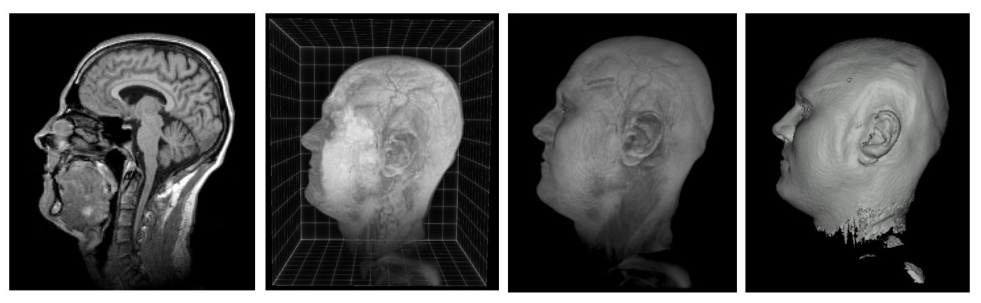
Intuitively grasping 3-D shapes requires visualisation of the whole object.
This is not possible when just looking at one or several slices of a 3-D data set.
Thus is it important about different volume rendering techniques that can create a 3-D appearance of the whole image.
This is especially useful for sparse data, where individual 2-D slices only contain a small subset of the relevant information.
Prerequisites
Before starting this lesson, you should be familiar with:
After completing this lesson, learners should be able to:
Understand the concepts and some methods of 3-D rendering.
Appreciate that 3-D rendering can be challenging for some data.
Perform basic volume rendering using a software tool.
Concept map
graph TD
D("3-D image data") --> R("Volume rendering")
R --> A("2-D image with 3-D appearance")
R -->|"Virtual Reality"| AA("Two 2-D images (one per eye)")
R ---|has| M("Many methods and settings...")
Open a 3D image of choice (see above for a list of example images)
Plugins > 3D Viewer
Explore rendering modes Edit > Display as
Volume: Volume rendering
Edit > Transfer function
Transparency: Channel: Alpha
Iso-Surface: Surface
Edit > Adjust threshold
Edit > Change color
skimage napari
###
# To create an animation of the volume the napari-animation plugin is needed.
# pip install napari-animation
###
importnumpyasnpfromskimage.ioimportimreadimportnapari# Read the image
# image = imread('https://github.com/NEUBIAS/training-resources/raw/master/image_data/xyzt_8bit__starfish_chromosomes.tif')
# image = imread('https://github.com/NEUBIAS/training-resources/raw/master/image_data/xyzc_8bit__em_synapses_and_labels.tif')
image=imread('https://github.com/NEUBIAS/training-resources/raw/master/image_data/xyz_8bit_calibrated__mri_full_head.tif')# image = imread('https://github.com/NEUBIAS/training-resources/raw/master/image_data/xyz_8bit_calibrated__organoid_nuclei.tif')
# image = imread('https://github.com/NEUBIAS/training-resources/raw/master/image_data/xyz_8bit_calibrated__fib_sem_crop.tif')
# image = imread('https://github.com/NEUBIAS/training-resources/raw/master/image_data/xyz_8bit_calibrated_labels__platy_tissues.tif')
# Check image type and values
print(image.dtype)print(np.min(image),np.max(image))print(image.shape)# Instantiate the napari viewer
viewer=napari.Viewer()# View the intensity image as grayscale
viewer.add_image(image,name='image',colormap='gray')# Napari GUI: choose a colormap according to the data type
# Napari GUI: change viewer from 2D to 3D, zoom in and out and rotate the volume
# Note: these values are optimized for xyz_8bit_calibrated__mri_full_head.tif
viewer.dims.ndisplay=3viewer.camera.zoom=2viewer.camera.angles=(0,-60,90)# Napari GUI: use rendering (and attenuation) modes
# Parameters can be changed for reproducibility
viewer.layers['image'].rendering='attenuated_mip'viewer.layers['image'].attenuation=1.# Take a screenshot of the scene created
fromnapari.utilsimportnbscreenshotnbscreenshot(viewer)# Acquire the frame as numpy array and add it to the napari GUI
screenshot=viewer.screenshot()viewer.add_image(screenshot,name='screenshot')viewer.dims.ndisplay=2# Napari GUI: realize this is a 2D RGBA image and can be saved as a PNG for presentations
print(screenshot.dtype)print(np.min(screenshot),np.max(screenshot))print(screenshot.shape)# Napari GUI: use napari-animation (https://github.com/napari/napari-animation) to create an animation of the volume
# %%
# Close the viewer (CI test requires this)
viewer.close()
Load an image using File > Open File(s)... or press Ctrl+O. One can also drag and drop an image into the GUI area to open it
Change viewer from 2D to 3D
zoom in and out (mouse scroll)
rotate the volume (pressing and holding left-click of mouse)
pan (Shift + pressing and holding left-click of mouse)
Add axes by clicking on View > Axes > Axes Visible
Add scale bar by clicking on View > Scale Bar > Scale Bar Visible
Open the same image in Fiji and note down the calibration given in Image > Properties...
Add the scale by opening a console within napari GUI and type this:
viewer.layers[viewer.layers[0].name].scale = [z, y, x]
where, x , y and z are scaling factors in their respective dimensions. Set this according to the metadata (i.e. the calibration noted down in the previous step) of the image.
Note(IMPORTANT): the above command viewer.layers[0].name only works if you have loaded just one image in napari
Try different rendering modes: mip, iso, attenuated_mip
Assessment
True or False
Surface rendering and volume rendering are identical words for the same 3-D visualisation method.
Volume rendering is particularly useful for data containing very dense 3-D information such as very many cells or nuclei in an organ of a biological specimen.
Volume rendering is a simple algorithm that can easily be used without expert knowledge.
Volume rendering is very useful to get an impression of the morphology and spatial distribution of objects.
Solution
False. Although both methods are used for 3-D rendering they are different. In surface rendering one needs to define “the shell” of an object and only this will be visible. In volume rendering the intensity of all voxels can be represented such as in a maximum intensity projection based volume rendering.
False. If the data is very dense, there is a high probabilty that no matter from which angle you look there will be objects hidden behind other objects. Thus, sparse data can be more suited to 3-D rendering than very dense data.
False. In fact, volume rendering is very complex and there are many things to learn to master it (see for example this website.
True. If the sample is not too dense, volume rendering allows one to get a quick overview of the whole 3-D specimen and its morphology.