The measurement of intensities in biological images is very common, e.g. to quantify expression levels of certain proteins by means of immuno-histochemistry. However, performing correct intensity measurements is very tricky and there are a lot of pitfalls. It is thus of utmost important to understand very well what one is doing. Without in-depth understanding the chance to publish wrong results based on intensity measurements is rather high.
Prerequisites
Before starting this lesson, you should be familiar with:
After completing this lesson, learners should be able to:
Understand the correct biophysical interpretation of the most common object intensity measurements
Perform object intensity measurements, including background subtraction
Concept map
graph TD
li[Object regions] --> im("Object intensity measurements")
ii[Intensity image] --> im
im --> table["Objects table oid | sum | mean | mean_bg 001 | 222 | 24 | 12 002 | 500 | 21 | 12 "]
style table text-align:left
ii --> bgm("Background measurement")
bgm --> table
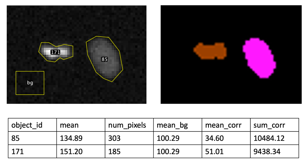
Figure
H2b-mCherry widefield image of two cells with common object and background intensity measurements, using manually drawn regions and/or a label mask image to delineate the objects.
Nomenclature
median
mean = average
sum = total = integrated
bg = background
Formula
mean_corr = mean - bg
sum_corr = mean_corr * num_pixels = ( mean - bg ) * num_pixels = sum - ( bg * num_pixels )
Biophysical interpretation
mean often resembles the concentration of a protein
sum often represents the total expression level of a protein
For the correct biophysical interpretation you need to know the PSF of your microscope.
More specifically, you need to know how the 3D extend of the PSF relates to 3D extend of your biological structures of interest. Essentially, you need to exactly know where your microscope system is measuring the intensities.
It is thus critical whether you used a confocal or a widefield microscope, because widefield microscope have an unbounded PSF along the z-axis.
Key points
Intensity measurements are generally very tricky and most likely the source of many scientific mistakes.
Please consider consulting a bioimage analysis expert.
Intensity measurements need a background correction.
Finding the correct background value can be very difficult and sometimes even impossible and, maybe, the project just cannot be done like this!
At least, think carefully about whether the mean or sum intensity is the right readout for your biological question.
If you publish or present something, label your measurement properly, e.g. “Sum Intensity” (just “Intensity” is not enough)!
Measure the mean and max intensities as well as the objects’ pixel area.
Make sure to also measure the mean intensity in the background and record this information
Export the results as a table and open in a spreadsheet software
Compute new columns for background corrected mean, max, and sum intensity.
Discuss the measurements’ biophysical interpretation
Repeat the activity using larger object regions
Due to the diffraction blur there is some subjectivity to how excatly to delineate the objects. Thus is is useful to compare how the measured values change when using larger regions.
Change LUT to see the noise in the background: [ Ctrl/Cmd + C ]
Draw a ROI in the background
[ Analyze › Set Measurements… ]
Mean gray value
Median
[ Analyze › Measure ]
Open the object intensity measurements table in a spreadsheet software (e.g. Excel or R)
Add the manual background measurment as a new column
Add new columns for background corrected sum and mean intensity
skimage napari
# %%
# Measure intensities with background subtraction
# %%
# Import python packages
fromOpenIJTIFFimportopen_ij_tiff,save_ij_tifffromskimage.ioimportimsaveimportnumpyasnpfromnapari.viewerimportViewerimportpandasaspdfromskimage.measureimportregionprops_table,regionprops# %%
# Load image and segmentation (aka labels)
image,*_=open_ij_tiff("https://github.com/NEUBIAS/training-resources/raw/master/image_data/xy_16bit__h2b.tif")labels,*_=open_ij_tiff("https://github.com/NEUBIAS/training-resources/raw/master/image_data/xy_8bit_labels__h2b.tif")print("labels",np.unique(labels))# %%
# Create a napari_viewer and visualize image and labels
viewer=Viewer()viewer.add_image(image)viewer.add_labels(labels)# %%
# Napari:
# Add a dedicated background label
# - Intensity measurements require background subtraction, thus one needs a region to measure the background intensity
# - Finding a suitable background region can be challenging, here we do it manually
# - Using the `layer controls` for the `labels` layer, manually create an additional label ("3" in this case) that specifically measures the background
# %%
# Appreciate that the labels image has been modified "in place"
# as there is now another "3" label
print("labels",np.unique(labels))# %%
# Check which intensity measurements are available
regionprops?# %%
# Measure the object intensities
# - This immediately converts the measurements into a pandas dataframe
df=pd.DataFrame(regionprops_table(labels,intensity_image=image,properties=('label','area','intensity_mean','intensity_max')))print(df)# %%
# Fetch the mean background intensity value
background=df.intensity_mean[2]print(background)# %%
# Append the sum intensity and
# background-corrected values to the table
df['intensity_sum']=df.intensity_mean*df.areadf['intensity_mean_corr']=df.intensity_mean-backgrounddf['intensity_max_corr']=df.intensity_max-backgrounddf['intensity_sum_corr']=df.intensity_mean_corr*df.areaprint(df)# Export the data
df.to_csv("intensity_measurements.csv")# %%
# Optional: Repeat the above with "https://github.com/NEUBIAS/training-resources/raw/master/image_data/xy_8bit_labels__h2b_dilate_labels.tif"
# - Discuss how the measurements are affected by the larger object regions
# %%
# Close the viewer (CI test requires this)
viewer.close()
Measure the both the mean and sum intensity of the NUP for each nucleus
Don’t forget to measure and take into account the image background
Think about the biophysical meaning of the mean and sum intensity.
Solution
Label
Mean
NumberOfVoxels
BG
Mean_corr
Sum_corr
1
34.3762
2092
25
9.38
19622
2
31.9296
2343
25
6.93
16236
3
32.4747
1342
25
7.47
10024
Interpretation of the mean intensity: The label masks seem generally wider than the nuclear envelope, thus an interpreation of the mean intensity as the local NUP density on the membrane is problematic. However, if the width of the label masks is kept constant across the experiment the mean intensity could indeed be a number that is proportional to the NUP density.
Interpretation of the sum intensity: The sum intensity is very much affected by the size of the measured region. It could be that in this image the nuclei were optically sectioned at different z-positions, cutting a more or less big region out of the nucleus. The sum intensity seem thus not very useful here.
Measure background intensity by drawing an ROI and [ Analyze > Measure ]
Measure the corrected mean and sum intensity using the formulas given in the main text of this module
Display the label image on top of the intensity image using an Overlay ([Image > Overlay > Add Image…]).
Based on this overlay, do you think the quantification of the signal of one of the nuclei may be problematic?
Solution
The label mask for label 3 also includes regions that are probably not part of the nuclear membrane and all intensity measurements may be affected by this.
Assessment
Fill in the blanks (discuss with your neighbour)
Fill in the blanks, using these words: number of pixels, integrated, mean, decrease, increase, increase, sum, decrease
Average intensity is just another word for ____ intensity.
Sum intensity is sometimes also called ____ intensity.
The ____ intensity is equal to the mean intensity times the ____ in the measured region.
In an unsigned integer image, increasing the size of the measurement region can only _____ the sum intensity.
In an unsigned integer image, decreasing the size of the measurement region can ____ or ____ the mean intensity.
In a floating point image, increasing the size of the measurement region could ____ the sum intensity.