After completing this lesson, learners should be able to:
Create an image analysis workflow comprising image denoising and object filtering.
Motivation
Finding objects in images typically presents itself with two challenges. First, the input image may not lend itseld to a simple intensity thresholding operation for binarisation. Second, there may be unwanted objects in the image such as hot pixels or objects that are not fully in the image. The first challenge typically is tackled by applying appropriate image filters to the raw data. The second challenge is tackled by defining and applying reproducible criteria to remove certain objects from the image.
Concept map
graph TD
GI["Grayscale input image"] --> FGI["Filtered grayscale image"]
FGI -->|has property|P["Interesting stuff is bright"]
FGI --> BI["Binary image"]
BI --> LI["Label image"]
LI --> FLI["Subset label image"]
FLI -->|has property|U["Unwanted labels are removed"]
FLI --> S("Shape measurement")
S --> SFT["Object feature table"]
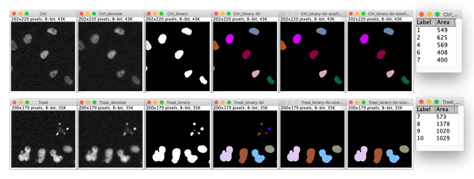
Figure
Nuclei segmentation and area measurement, including image denoising and object filtering.
Workflow:
Apply the workflow outlined above (see Concept map and Example figure) to both images. The modules listed in this module’s Prerequisites contain the information as to how to conduct each step of the workflow. You can try different filters on the image for denoise (e.g. mean, gaussian, …)
# %%
# Import modules
importnaparifromOpenIJTIFFimportopen_ij_tiff,save_ij_tifffromskimage.filters.rankimportmeanfromskimage.morphologyimportdisk,remove_small_objects,remove_small_holesfromskimage.measureimportlabel,regionprops_tablefromskimage.segmentationimportclear_borderimportpandasaspdimportosimportnumpyasnp# %% [markdown]
# ### Process the first image
# %%
# Instantiate the napari viewer
viewer=napari.Viewer()# Read and inspect the image:
fpath='https://github.com/NEUBIAS/training-resources/raw/master/image_data/xy_8bit__nuclei_noisy_small.tif'image,axes_image,scales_image,units_image=open_ij_tiff(fpath)viewer.add_image(image)# %%
# Apply local mean filter
radius=3disk_radius=disk(radius)denoised_image=mean(image,disk_radius)viewer.add_image(denoised_image)# %%
# Binarize the image:
thr=25binary_image=denoised_image>thrviewer.add_labels(binary_image)# %%
# Fill small holes
min_size_holes=100filled_binary_image=remove_small_holes(binary_image,area_threshold=min_size_holes)viewer.add_labels(filled_binary_image)# %%
# Find labels
connectivity=2label_mask=label(filled_binary_image,connectivity=connectivity)viewer.add_labels(label_mask)# %%
# Remove small regions
min_size_regions=100filtered_label_mask=remove_small_objects(label_mask,min_size=min_size_regions)viewer.add_labels(filtered_label_mask)# %%
# Remove regions touching the borders
filtered_label_mask_no_borders=clear_border(filtered_label_mask)viewer.add_labels(filtered_label_mask_no_borders)# %%
# Print areas for each cell:
properties=pd.DataFrame(regionprops_table(filtered_label_mask_no_borders,properties={'label','area'}))print(properties)# %%
# Find the basename of the input file from input file path
file_name=os.path.basename(fpath)base_name=os.path.splitext(file_name)[0]print(base_name)# %%
# Save final label mask as tif file
mask_save_name=base_name+"_labelmask.tif"save_ij_tiff(mask_save_name,filtered_label_mask_no_borders.astype(np.uint8),axes_image,scales_image,units_image)print(f"The label mask is saved as : {mask_save_name}")# %%
# Save object properties dataframe as csv file
table_save_name=base_name+"_intensity_measurements.csv"properties.to_csv(table_save_name,index=False)print(f"The object properties are saved as : {table_save_name}")# %%
# Repeat the steps on the second image
# %%
# Close the viewer (CI test requires this)
viewer.close()