Detecting a set of objects in an image, counting them and measuring certain characteristics about their morphology is probably the most frequently occurring task in bioimage analysis. Depending on the image, even this task could become quite challenging and the workflow could become quite complex. Here we start with a relatively simple image where combining a minimal set of image analysis components into a simple workflow does the job.
Prerequisites
Before starting this lesson, you should be familiar with:
The images are two time points of a time lapse experiment where the INCENP gene was subjected to siRNA knock-down. The data are taken from the published mitocheck screen. In this screen the authors carried out a genome-wide phenotypic profiling of each of the ~21,000 human protein-coding genes by two-day live imaging of fluorescently labelled chromosomes. Phenotypes were scored quantitatively by computational image processing, which allowed them to identify hundreds of human genes involved in diverse biological functions including cell division, migration and survival. The analysis that we apply here is, of course, simpler than what the authors did in the publication, but the essence is already very similar. In addition, to simplify the task we work here on images that were cropped and slightly denoised.
Workflow
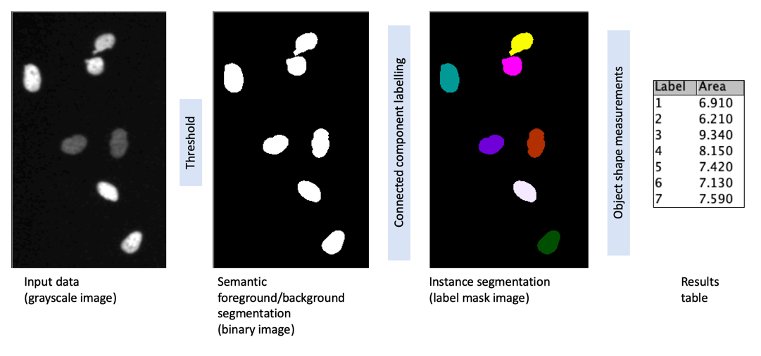
Open the image
Apply a threshold to create a binary image
Apply a connected component analysis on the binary image to create a label mask image
On the label mask image preform object shape measurements
Save the label mask image, e.g. as TIFF file
Save the shape measurements, e.g. as CSV file
Notes
When writing code to implement the above workflow it is recommended to put the analysis workflow into a function that can then be called during batch analysis of many images.
The modules listed in “Prerequisites” contain the information as to how to conduct each step of the workflow.
The nuclei in both images look quite different. Find shape measurements that quantify this.
The workflow contains a thresholding step; choosing this threshold is somewhat arbitrary; try different thresholds and explore how this affects the measurements.
Show activity for:
ImageJ GUI
Process › Binary › Options...
[X] Black background, because we work with fluorescence data
Open one of the above images
Image › Duplicate...
Title = binary
Draw a line profile to find a good threshold
Use the straight line tool in the Fiji menu bar
Analyze › Plot Profile
Live and move the line around, including nuclei and background pixels
Image › Adjust › Manual Threshold...
Min = 25
Max = 255, because this is the maximum of the image data-type
type = 8 bits, because we will have less than 255 objects
Plugins › MorphoLibJ › Analyze › Analyze Regions
You may subset the measurements if you are not interested in all
ImageJ Macro
/**
* 2D Nuclei segmentation (simple workflow)
*
* Requirements:
* - Update site: IJPB-Plugins (MorpholibJ)
*
*/// Threshold parameter// Exercise: Explore how choosing a different threshold value affects the measured shapes threshold=25;// Coderun("Close All");run("Options...","iterations=1 count=1 black do=Nothing");analyseNuclei("INCENP_T1","https://github.com/NEUBIAS/training-resources/raw/master/image_data/xy_8bit__mitocheck_incenp_t1.tif",threshold);analyseNuclei("INCENP_T70","https://github.com/NEUBIAS/training-resources/raw/master/image_data/xy_8bit__mitocheck_incenp_t70.tif",threshold);run("Tile");functionanalyseNuclei(name,filePath,threshold){open(filePath);rename(name);setMinAndMax(0,100);run("Duplicate...","title="+name+"_binary");setThreshold(threshold,65535);run("Convert to Mask");run("Connected Components Labeling","connectivity=4 type=[8 bits]");run("glasbey_on_dark");run("Analyze Regions","area");}
skimage and napari
# %% [markdown]
# ## Workflow segment 2D nuclei
# This activity is part of [Nuclei segmentation and shape measurement](https://neubias.github.io/training-resources/workflow_segment_2d_nuclei_measure_shape/index.html)
# %%
# Import modules
importnaparifromOpenIJTIFFimportopen_ij_tifffromskimage.measureimportlabel,regionprops_tableimportpandasaspd# %%
# Instantiate the napari viewer
viewer=napari.Viewer()# %%
# Open and inspect the image
# Learning opportunity: change file_path and the name of the image to analyse a different image: https://github.com/NEUBIAS/training-resources/raw/master/image_data/xy_8bit__mitocheck_incenp_t70.tif
file_path="https://github.com/NEUBIAS/training-resources/raw/master/image_data/xy_8bit__mitocheck_incenp_t1.tif"image,axes,scales,units=open_ij_tiff(file_path)viewer.add_image(image,name='incenp_t1')# %%
# Binarize the image
# Learning opportunity: explore different threshold values
image_binary=image>25viewer.add_image(image_binary,name='binary',opacity=0.3)# %%
# Learning opportunity: explore [automatic thresholding](https://scikit-image.org/docs/stable/api/skimage.filters.html), e.g. `skimage.filters.threshold_li`
# %%
# Perform connected components analysis (i.e create labels)
image_labels=label(image_binary)viewer.add_labels(image_labels,name='labels')# %%
# Measure nuclei shapes
properties=regionprops_table(image_labels,properties={'label','area'})# %%
# Learning opportunity: Try also different measurements. See documentation of [skimage regionsprops](https://scikit-image.org/docs/stable/api/skimage.measure.html#skimage.measure.regionprops)
# %%
# Print areas for each cell
# Learning opportunity: print other measurements
properties_dataframe=pd.DataFrame(properties)print(properties_dataframe)# %%
# Learing opportunity: Generalize the workflow for many images
#
# A "for loop*"" allows to extend the workflow to many more images and fully automate it. Here the backbone of code
# ```
# image_paths = ["https://github.com/NEUBIAS/training-resources/raw/master/image_data/xy_8bit__mitocheck_incenp_t1.tif", "https://github.com/NEUBIAS/training-resources/raw/master/image_data/xy_8bit__mitocheck_incenp_t70.tif"]
#
# for file_path in image_paths:
# print(file_path)
# image, axes, scales, units = open_ij_tiff(file_path)
# # More code here
# ```
#
# Save the data: Ideally one would like to save the results of each processed image. For saving the label image you can use [`skimage.io.imsave`](https://scikit-image.org/docs/stable/api/skimage.io.html#skimage.io.imsave) for saving the table you can use e.g. [`pandas.DataFrame.to_csv`](https://pandas.pydata.org/docs/reference/api/pandas.DataFrame.to_csv.html), i.e. `properties_dataframe.to_csv`. You can add these functions within the for loop.
#
# To save the data one needs unique names. For instance one could extract the name of the image using [`os.path`](https://docs.python.org/3/library/os.path.html) functionality and then add some additional identifiers.
# %%
# Close the viewer (CI test requires this)
viewer.close()
CellProfiler
Ensure you have access to CellProfiler version 4.2.8