After completing this lesson, learners should be able to:
Understand how objects in images are represented as a label mask image.
Apply connected component labeling to a binary image to create a label mask image.
Motivation
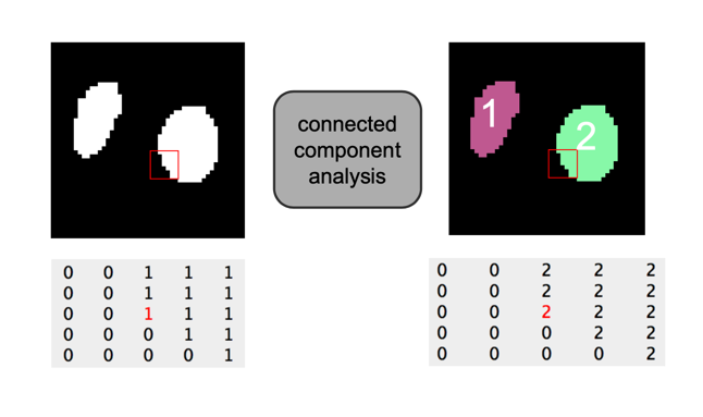
A main task of bioimage analysis is to detect objects in images. To do so one needs to be able to label pixels that are part of the same object in a way that this can be efficiently stored and processed by the computer. A prevalent way of doing this is connected component labeling, which is discussed in this module.
Concept map
graph TD
BI("Binary image") -->|input|CC("Connected component analysis")
C("Connectivity") -->|parameter|CC
OD("Output data type") -->|parameter|CC
CC -->|output|LI("Label image")
LI -->|display with|MCL("Multi color LUT")
LI -->|content|PV("Integer pixel values")
PV --> BG("0: Background")
PV --> R1("1: Region 1")
PV --> R2("2: Region 2")
PV --> R3("...")
Inspect the pixel values of the label image and see what you can learn about the objects that are encoded in this image.
Show activity for:
ImageJ MorpholibJ Macro & GUI
// 3D connected components labeling (6-connected)open("https://github.com/NEUBIAS/training-resources/raw/master/image_data/xyz_8bit_binary__spots.tif");rename("binary");run("Connected Components Labeling","connectivity=6 type=[8 bits]");run("glasbey_on_dark");setMinAndMax(0,255);// Note: surprisingly this determines the content of below histogram!run("Histogram","stack");
skimage napari
# %% [markdown]
# # 3D connected component labeling
# %%
# Import modules
importnaparifromskimage.measureimportlabelfromOpenIJTIFFimportopen_ij_tiffimportnumpyasnp# %%
# Instantiate the napari viewer
viewer=napari.Viewer()# %%
# Read a binary 3D image and display it
binary_3D_image,axes_binary_3D_image,scales_binary_3D_image,units_binary_3D_image=open_ij_tiff('https://github.com/NEUBIAS/training-resources/raw/master/image_data/xyz_8bit_binary__spots.tif')viewer.add_image(binary_3D_image)# %%
# Connected components with connectivity 2 (aka 3D 26 connectivity)
labels_3D_conn2_image=label(binary_3D_image,connectivity=2)viewer.add_labels(labels_3D_conn2_image)# %%
# Interrogate the values in the 3D label image
print(np.unique(labels_3D_conn2_image))# the object indices
print(len(np.unique(labels_3D_conn2_image))-1)# the number of objects (minus background)
print(np.max(labels_3D_conn2_image))# the number of objects (minus background) (if the labels are consecutive!)
np.sum(labels_3D_conn2_image==2)# the number of pixels (~volume) in object number 2
# %%
# %% [markdown]
# # Many objects
# %%
# Import modules
importnaparifromskimage.measureimportlabelfromOpenIJTIFFimportopen_ij_tiffimportnumpyasnp# %%
# Instantiate the napari viewer
viewer=napari.Viewer()# %%
# Read a binary 2D image and display it
fpath="https://github.com/NEUBIAS/training-resources/raw/master/image_data/xy_8bit_binary__many_vesicles.tif"binary_2D_image,axes_binary_2D_image,scales_binary_2D_image,units_binary_2D_image=open_ij_tiff(fpath)viewer.add_image(binary_2D_image)# %%
# Connected components with connectivity 1
labels_2D_conn1_image=label(binary_2D_image,connectivity=1)viewer.add_labels(labels_2D_conn1_image)# %%
# Interrogate the values in the 2D label image
print(np.unique(labels_2D_conn1_image))# the object indices
print(len(np.unique(labels_2D_conn1_image))-1)# the number of objects (minus background)
print(np.max(labels_2D_conn1_image))# the number of objects (minus background) (if the labels are consecutive!)
# %%
Assessment
Fill in the blanks
Fill in the blanks, using these words: less, larger, 6, 255, 4, more.
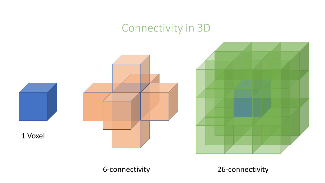
In 3D, pixels have _____ neighbors than in 2D.
8-connected connectivity results in _____ objects than 4-connected connectivity.
In 3D, pixels have __ non-diagonal neighbors.
In 2D, pixels have __ non-diagonal neighbors.
A 8-bit label mask image can have maximally _____ objects.
The maximum value in a label mask image is equal to or _____ than the number of objects.
Solution
more
less
6
4
255
larger
Explanations
Typically, one first categorise an image into background and foreground regions, which can be represented as a binary image. Such clusters in the segmented image are called connected components. The relation between two or more pixels is described by its connectivity. The next step is a connected components labeling, where spatially connected regions of foreground pixels are assigned (labeled) as being part of one region (object).
In an image, pixels are ordered in a squared configuration.
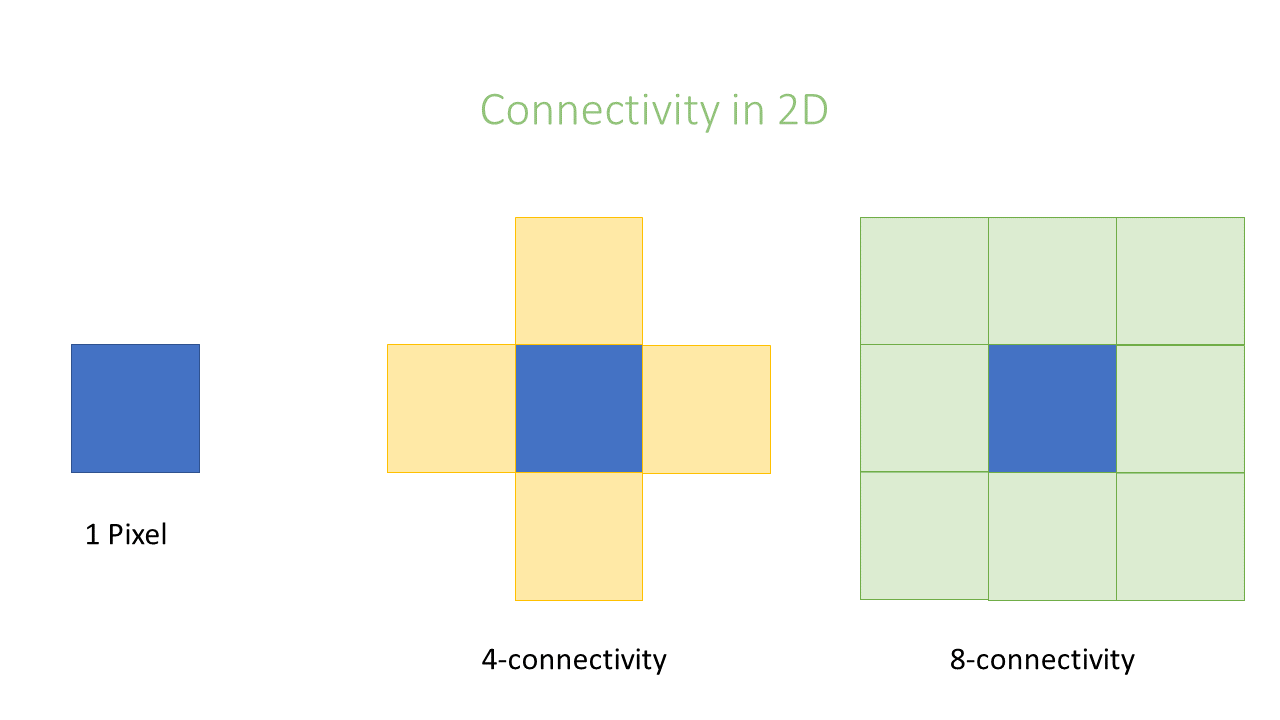
For performing a connected component analysis, it is important to define which pixels are considered direct neighbors of a pixel. This is called connectivity and defines which pixels are considered connected to each other.
Essentially the choice is whether or not to include diagonal connections.
Or, in other words, how many orthogonal jumps to you need to make to reach a neighboring pixel; this is 1 or an orthogonal neighbor and 2 for a diagonal neighbor.
This leads to the following equivalent nomenclatures: