Automatic thresholding
Overview
Teaching: min
Exercises: minQuestions
Objectives
Understand how an image histogram can be used to derive a threshold
Apply automatic threshold to distinguish foreground and background pixels
Key points
- Most auto thresholding methods do two class clustering
- If the histogram is bimodal, most automated methods will perform well
- If the histogram has more than two peaks, automated methods could produce noisy results
Key Points
Batch exploration of segmentation results
Overview
Teaching: min
Exercises: minQuestions
Objectives
Use various tools to efficiently inspect segmented images and corresponding object measurements.
Key Points
Big image data formats
Overview
Teaching: min
Exercises: minQuestions
Objectives
Understand the concepts of lazy-loading, chunking and scale pyramids
Understand some file formats that implement chunking and scale pyramids
Similarities of big microscopy data with Google maps
We can think of the data in Google maps as one very big 2D image. Loading all the data in Google maps into your phone or computer is not possible, because it would take to long and your device would run out of memory.
Another important aspect is that if you are currently looking at a whole country, it is not useful to load very detailed data about individual houses in one city, because the monitor of your device would not have enough pixels to display this information.
Thus, to offer you a smooth browsing experience, Google Maps lazy loads only the part of the world (chunk) that you currently look at, at an resolution level that is approriate for the number of pixels of your phone or computer monitor.
Chunking
The efficiency with which parts (chunks) of image data can be loaded from your hard disk into your computer memory depends on how the image data is layed out (chunked) on the hard disk. This is a longer, very technical, discussion and what is most optimal probably also depends on the exact storage medium that you are using. Essentially, you want to have the size of your chunks small enough such that your hardware can load one chunk very fast, but you also want the chunks big enough in order to minimise the number of chunks that you need to load. The reason for the latter is that for each chunk your software has to tell your computer “please go and load this chunk”, which in itself takes time, even if the chunk is very small. Thus, big image data formats typically offer you to choose the chunking such that you can optimise it for your hardware and access patterns.
Resolution pyramids
If the image data is big and one is zoomed out, the data may have more pixels that the viewing window of your computer monitor. In this case it makes no sense to load all the data, but a lower resolution (down-sampled) version of the same data would give you the same displayed information and, since it is less data, it could be loaded faster. Thus, for big image data one typically saves the data multiple times at different levels of downsampling in a so-called resolution pyramid. If you use appropriate viewing software it will automatically load the data from the appropriate resolution level, depending on your zoom level and the number of pixels of your viewing device. Note that is not only useful for fast visualisation, but can be also handy for image analysis purposes, where certain computations may not need to be performed on the full resolution data.
See also an introduction to resolution pyramids on Wikipedia
TIFF chunking
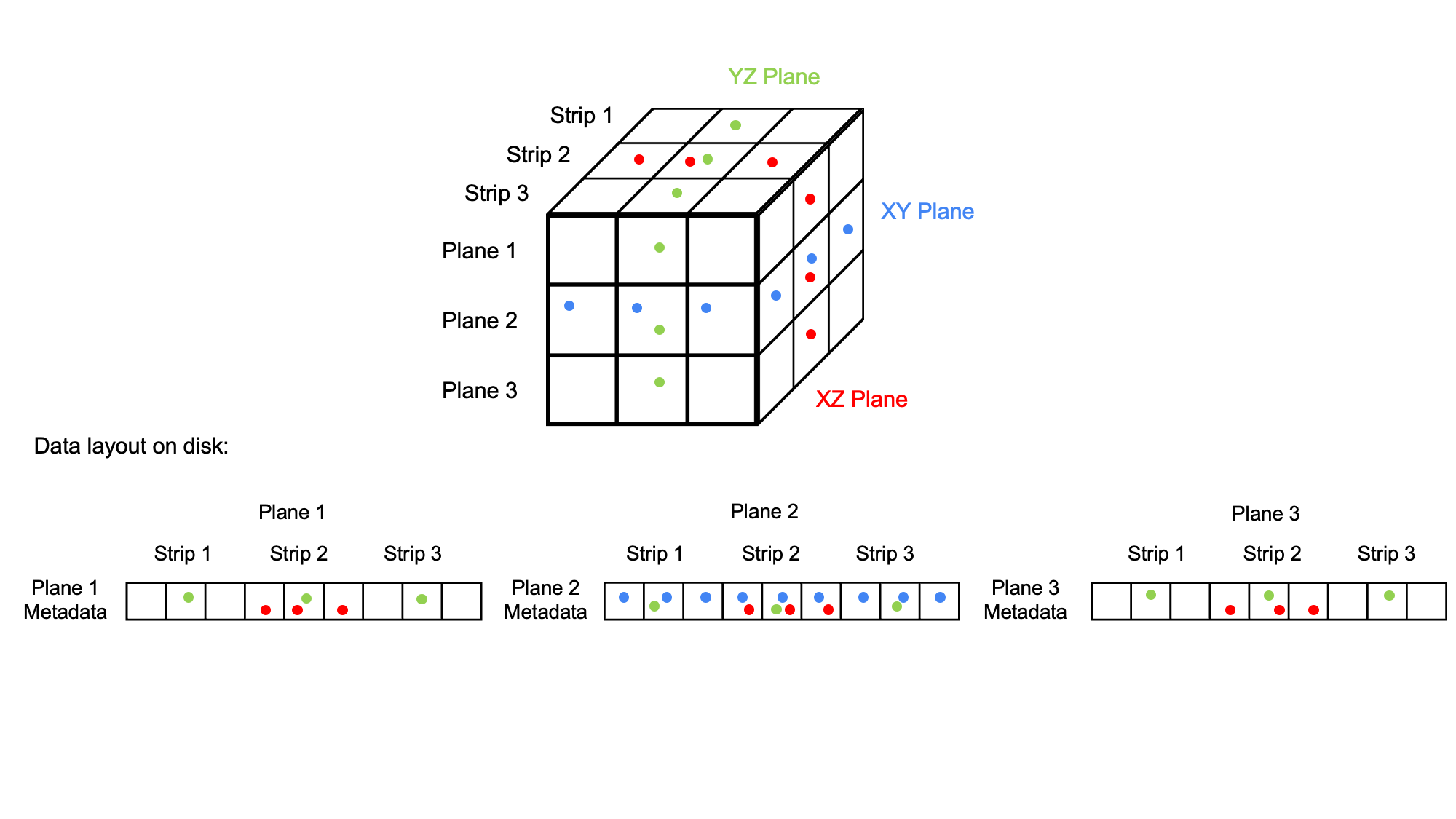
TIFF files are chunked as planes and as strips within the planes. One can therefore efficiently lazy load XY planes from a TIFF file. However, in particular lazy loading of YZ planes is very inefficient. The reason is that for typical storage systems (e.g., hard disks) data that resides close together can be swiftly fetched in one read operation. However, data that is distributed must be read in several seek and read operations, which is much slower, because each operation needs time. Note that often it is actually faster to just read everything in one go, even if not all data is needed.
Key Points
Cloud based batch analysis
Overview
Teaching: min
Exercises: minQuestions
Objectives
Understand how to leverage cloud computing platforms, such as Galaxy, for efficient bioimage batch analysis
Key Points
Cloud based interactive analysis
Overview
Teaching: min
Exercises: minQuestions
Objectives
Understand interactive analysis platforms, including virtual desktops, Galaxy interactive tools, and Jupyter notebooks for bioimage analysis.
Run bioimage tools, such as CellPose on virtual desktops
Run Galaxy Interactive Tools for bioimage analysis
Key Points
Connected component labeling
Overview
Teaching: min
Exercises: minQuestions
Objectives
Understand how objects in images are represented as a label mask image
Apply connected component labeling to a binary image to create a label mask image
Typically, one first categorise an image into background and foreground regions, which can be represented as a binary image. Such clusters in the segmented image are called connected components. The relation between two or more pixels is described by its connectivity. The next step is a connected components labeling, where spatially connected regions of foreground pixels are assigned (labeled) as being part of one region (object).
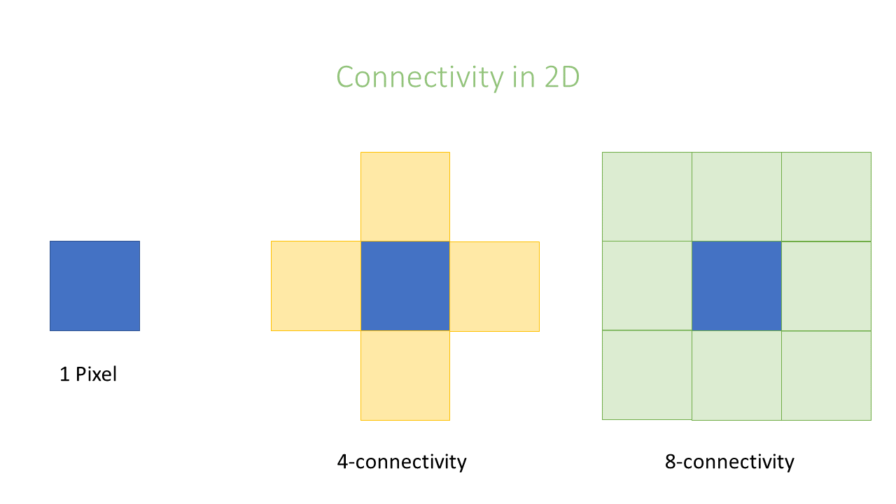
In an image, pixels are ordered in a squared configuration.
For performing a connected component analysis, it is important to define which pixels are considered direct neighbors of a pixel. This is called connectivity and defines which pixels are considered connected to each other.
Essentially the choice is whether or not to include diagonal connections.
Or, in other words, how many orthogonal jumps to you need to make to reach a neighboring pixel; this is 1 or an orthogonal neighbor and 2 for a diagonal neighbor.
This leads to the following equivalent nomenclatures:
- 2D: 1 connectivity = 4 connectivity
- 2D: 2 connectivity = 8 connectivity
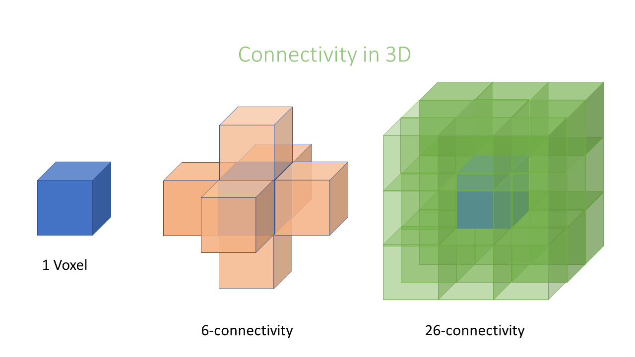
- 3D: 1 connectivity = 6 connectivity
- 3D: 2 connectivity = 26 connectivity
Key Points
Convolutional filters
Overview
Teaching: min
Exercises: minQuestions
Objectives
Understand the basic principle of a convolutional filter.
Apply convolutional filters to an image.
Key Points
Correlative image rendering
Overview
Teaching: min
Exercises: minQuestions
Objectives
Understand how heterogeneous image data can be mapped from voxel space into a global coordinate system.
Understand how an image viewer can render a plane from a global coordinate system.
Key Points
Data types
Overview
Teaching: min
Exercises: minQuestions
Objectives
Understand that images have a data type which limits the values that the pixels in the image can have.
Understand common data types such as 8-bit, 12-bit and 16-bit unsigned integer.
Image data types
The pixels in an image have a certain data type. The data type limits the values that pixels can take.
Unsigned integer data types
Many microscopes save their data in the unsigned integer datatype.
A pixel of an N-bit unsigned integer data can be between 0 and 2^N - 1.
For example
- 8-bit unsigned integer: 0 - 255
- 12-bit unsigned integer: 0 - 4095
- 16-bit unsigned integer: 0 - 65535
Intensity clipping (saturation)
If the value of a pixel in an N-bit unsigned integer image is equal to either 0 or 2^N - 1, you cannot know for sure whether you lost information at some point during the image acquisition or image storage.
For example, if there is a pixel with the value 255 in an unsigned integer 8-bit image, it may be that the actual intensity “was higher”, e.g. would have corresponded to a gray value of 302. One speaks of “saturation” or “intensity clipping” in such cases.
It is important to realise that there can be also clipping at the lower end of the range (some microscopes have an unfortunate “offset” slider that can be set to negative values, which can cause this). Typically, images with clipping at the lower feature large regions where all pixel values are 0. In general this is bad, because many image analysis operations (such as object intensity measurements) require knowledge of the background intensity of the image. This background intensity cannot be measured in images that are clipped.
Key Points
Digital image basics
Overview
Teaching: min
Exercises: minQuestions
Objectives
Understand that a digital image is represented as an N-dimensional array.
Practically visualise an image.
Practically quantitatively inspect the image (array) elements (pixels, voxels).
Digital image dimensions
There are several ways to describe the size of a digital image. For example, the following sentences describe the same image.
- The image has 2 dimensions, the length of dimension 0 is 200 and the length of dimension 1 is 100.
- The image has a size/shape of (200, 100).
- The image has 200 x 100 pixels.
Note that “images” in bioimaging can also have more than two dimensions and one typically specifies how to map those dimensions to the physical space (x, y, z, and t). For example, if you acquire a 2-D movie with 100 time points and each movie frame consisting of 256 x 256 pixels it is quite common to represent this as a 3-D array with a shape of (256, 256, 100) accompanied with metadata such as ( (“x”, 100 nm), (“y”, 100 nm), (“t”, 1 s) ); check out the module on spatial calibration for more details on this.
Key Points
Display settings
Overview
Teaching: min
Exercises: minQuestions
Objectives
Understand how the numerical pixel values of an image are transformed into bright and colorful images that you see on display screen.
Understand what a colormap is and why adjusting it is useful.
Understand how perception about image content changes on viewing it by altering contrast and colormaps
Use display settings responsibly for scientific purposes.
Colormaps do the mapping from a numeric pixel value to a color. This is the main mechanism how we visualize microscopy image data. In case of doubt, it is always a good idea to show the mapping as an inset in the image (or next to the image).
Nomenclature
Color mapping may have different names depending upon the software. Fiji uses the term “Look-up table (LUT)”, whereas MATLAB sticks to “colormap”. In some other communities/software, it is also called as “color transfer function”.
Single color colormaps
Single color colormaps are typically configured by choosing one color such as, e.g., grey or green, and choosing a min and max value that determine the brightness of this color depending on the value of the respective pixel in the following way:
brightness( value ) = ( value - min ) / ( max - min )
In this formula, 1 corresponds to the maximal brightness and 0 corresponds to the minimal brightness that, e.g., your computer monitor can produce.
Depending on the values of value, min and max it can be that the formula yields values that are less than 0 or larger than 1.
This is handled by assigning a brightness of 0 even if the formula yields values < 0 and assigning a brightness of 1 even if the formula yields values
larger than 1. In such cases one speaks of “clipping”, because one looses (“clips”) information about the pixel value (see below for an example).
Clipping example
min = 20, max = 100, v1 = 100, v2 = 200
brightness( v1 ) = ( 100 - 20 ) / ( 100 - 20 ) = 1
brightness( v2 ) = ( 200 - 20 ) / ( 100 - 20 ) = 2.25
Both pixel values will be painted with the same brightness as a brightness larger than 1 is not possible (see above).
Multicolor colormaps
As the name suggests multi color colormaps map pixel gray values to different colors.
For example:
0 -> black
1 -> green
2 -> blue
3 -> ...
Typical use cases for multicolor colormaps are images of a high dynamic range (large differences in gray values) and label mask images (where the pixel values encode object IDs).
Sometimes, also multicolor colormaps can be configured in terms of a min and max value. The reason is that multicolor colormaps only have a limited amount of colors, e.g. 256 different colors. For instance, if you have an image that contains a pixel with a value of 300 it is not immediately obvious which color it should get; the min and max settings allow you to configure how to map your larger value range into a limited amount of colors.
Key Points
Colormap turns numeric pixel values into colors/brightness on your screen.
A colormap has configurable contrast limits that determine the pixel value range that is rendered linearly to display the image.
Colormap settings must be responsibly chosen to convey the intended scientific message and not to hide relevant information.
A gray scale colormap is usually preferable; especially blue and red colormaps are not well visible for many people.
For high dynamic range images multicolor colormaps may be useful to visualize a wider range of pixel values.
Distance transform
Overview
Teaching: min
Exercises: Distance to center, ImageJ GUIdistance_transform/exercises/distance_transform_geodesic_imagejgui.mdGlial thickness, ImageJ GUIdistance_transform/exercises/distance_transform_skeldist_imagejgui.md minQuestions
Objectives
Understand how to use distance transform to quantify morphology of objects
Understand how to use distance transform to quantify distance between objects
Understand approximate nature of distance transform
Chamfer distance (modified from MorpholibJ Manual)
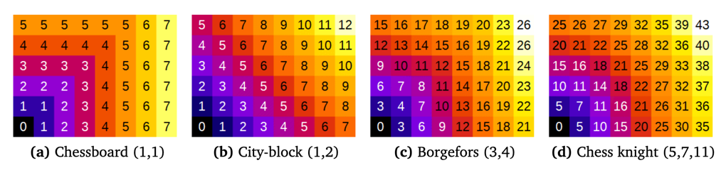
Several methods (metrics) exist for computing distance maps. The MorphoLibJ library implements distance transforms based on chamfer distances. Chamfer distances approximate Euclidean distances with integer weights, and are simpler to compute than exact Euclidean distance (Borgefors, 1984, 1986). As chamfer weights are only an approximation of the real Euclidean distance, some differences are expected compared to the actual Euclidean distance map.
Several choices for chamfer weights are illustrated in above Figure (showing the not normalized distance).
- The “Chessboard” distance, also named Chebyshev distance, gives the number of moves that an imaginary Chess-king needs to reach a specific pixel. A king can move one pixel in each direction.
- The “City-block” distance, also named Manhattan metric, weights diagonal moves differently.
- The “Borgefors” weights were claimed to be best approximation when considering the 3-by-3 neighborhood.
- The “Chess knight” distance also takes into account the pixels located at a distance from (±1, ±2) in any direction. It is usually the best choice, as it considers a larger neighborhood.
To remove the scaling effect due to weights > 1, it is necessary to perform a normalization step. In MorphoLibJ this is performed by dividing the resulting image by the first weight (option Normalize weights).
Key Points
Flat-field correction
Overview
Teaching: min
Exercises: minQuestions
Objectives
Formulate the mathematical relationship between the raw image and the corrected image
Evaluate methods to obtain a flat-field reference (calibration slide or retrospective computation)
Perform a flat-field correction and evaluate the results
Key Points
Global background correction
Overview
Teaching: min
Exercises: ImageJ Macro & GUIglobal_background_correction/exercises/global_background_correction.md minQuestions
Objectives
Measure the background in an image
Apply image math to subtract a background intensity value from all pixels and understand that the output image should have a floating point data type
Key Points
Illumination and shading artefacts
Overview
Teaching: min
Exercises: minQuestions
Objectives
Identify global shading patterns caused by e.g. Gaussian illumination
Understand implication for intensity measurements
Key Points
Image data formats
Overview
Teaching: min
Exercises: minQuestions
Objectives
Open various image files formats
Understand the difference between image data and metadata
Key Points
Imaging thick biological samples
Overview
Teaching: min
Exercises: minQuestions
Objectives
Understand that the geometry and optical properties of your biological specimen can have a large influence on the measured intensities
Key Points
Local background correction
Overview
Teaching: min
Exercises: minQuestions
Objectives
Understand how to use image filters for creating a local background image
Use the generated local background image to compute a foreground image
There exist multiple methods on how to compute a background image. Which methods and parameters work best depends on the specific input image and the size of the object of interest.
Common methods are:
- Median filtering
- Morphological opening. Subtraction of the opened image from the original image is also called Top-Hat filtering.
- Rolling ball, this alogorithm is implemented for instance in ImageJ
Background Subtractionorskimage.restoration.rolling_ball
Some of the methods may be sensistive to noise. Therefore, it can be convenient to smooth the image, e.g. with a mean or gaussian filtering, prior computing the background image.
Key Points
Median filter
Overview
Teaching: min
Exercises: minQuestions
Objectives
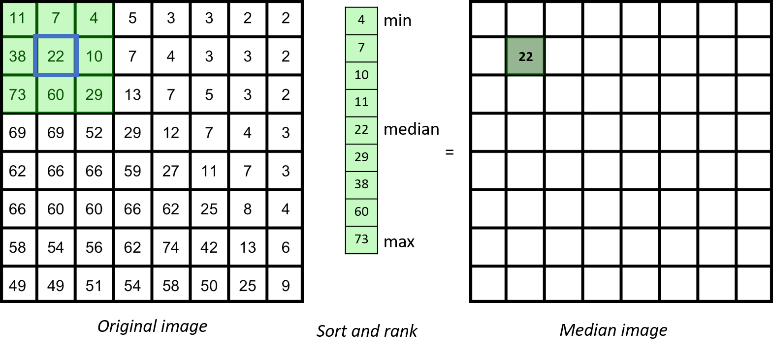
Understand in detail what happens when applying a median filter to an image
Properties of median filter
The median filter is based on ranking the pixels in the neighbourhood
In general, for any neighbourhood filter, if the spatial extend of the neighbourhood is significantly (maybe three-fold) smaller than the smallest spatial length scale that you care about, you are on the safe side.
However, in biology, microscopy images are often containing relevant information down to the level of a single pixel. Thus, you typically have to deal with the fact that filtering may alter your image in a significant way. To judge whether this may affect your scientific conclusions you therefore should study the effect of filters in some detail.
Although a median filter typically is applied to a noisy gray-scale image, understanding its properties is easier when looking at a binary image.
From inspecting the effect of the median filter on above test image, one could say that a median filter
- is edge preserving
- cuts off at convex regions
- fills in at concave regions
- completely removes structures whose shortest axis is smaller than the filter width
Key Points
Morphological filters
Overview
Teaching: min
Exercises: minQuestions
Objectives
Understand how to design morphological filters using rank filters
Execute morphological filters on binary or label images and understand the output
Rank filters
In the region defined by the structuring element, pixel elements are ranked/sorted according to their values. The pixel in the filtered image is replaced with the corresponding sorted pixel (smallest = min, greatest = max, median ). See also Median filter. Morphological filters corresponds to one or several rank filters applied to an image.
Morphological filters on binary images
A typical application of these filters is to refine segmentation results. A max-filter is called dilation whereas a min-filter is called erosion. Often rank filters are applied in a sequence. We refer to a closing operation as a max-filter followed by a min-filter of the same size. An opening operation is the inverse, a min-filter followed by a max-filter.
Opening operations will:
- Remove small/thin objects which extent is below the size of the structuring element
- Smooth border of an object
Closing operations:
- Fill small holes below the size of the structuring element
- Can connect gaps
Image subtraction using eroded/dilated images allows to identify the boundary of objects and is referred to morphological gradients:
- Internal gradient: original - eroded
- External gradient: dilated - original
- (Symmetric) gradient: dilated - eroded
Fill holes operation is a slightly more complex morphological operation. It is used to identify background pixels surrounded by foreground pixels and change their value to foreground. Algorithmically there are several ways to achieve this.
Morphological filters on label images
Morphological filters work also on label images. If the objects are not touching this will achieve the expected result for each label. However, when objects touch each other, operations such as dilations can lead to unwanted results.
Morphological filters on grey level images
Min and max operations can be applied to grey level images. Applications are for example contrast enhancement, edge detection, feature description, or pre-processing for segmentation.
Key Points
Multichannel images
Overview
Teaching: min
Exercises: minQuestions
Objectives
Understand/visualize different image channels.
Color combinations for multi channel images
General recommendationas
The choice of lookup tables to display a merged multi-channel image should fulfill:
- Distinct color separation so to maximize the visual separation between channels.
- Avoidance of problematic color combinations that can’t be distinguished with color vision deficiency (e.g. red/green)
- If unsure test color combinations using a “color-blind mode”. For example in ImageJ
Image > Color > Simulate Color Blindness - If possible show the single channels next to the merged channel for better clarity
Suggested color combinations
- Two channels:For example Green/Magenta, Blue/Yellow, Red/Cyan, Blue/Red
- Three channels: For example Magenta/Green/Blue, Megenta/Yellow/Cyan, Red/Cyan/Yellow
- More than three channels: Displaying the merged image with enough contrast is challenging. It depends on the structures that have been stained and how much they overlap. Different color combinations should be tried out. One possibiility is Magenta/Green/Yellow/Cyan, or a grayscale LUT for one or more of the reference (less important) channels.
Key Points
N-dimensional images
Overview
Teaching: min
Exercises: minQuestions
Objectives
Explore and view the different dimensions image data can have.
Key Points
Neighborhood filters
Overview
Teaching: min
Exercises: minQuestions
Objectives
Understand the basic principle of a neighborhood filter.
Apply basic neighborhood filters to an image.
Neighborhood filters comprise two ingredients: a definition of the pixel neighborhood (size and shape) and a mathematical recipe what to compute on this neighborhood. The result of this computation will be used to replace the value of the central pixel in the neighborhood. This procedure can be applied to several (all) pixels of an image to obtain a filtered image. The animation shows a square neighborhood (3x3) applied to the inner pixels of the image.
There are tons of different neighborhood filters, and you can also invent one!
The neighborhoods
The neighborhood of a pixel is also called a structuring element (SE) and can have various sizes and shapes. Here, we use one of the simplest and most widely used neighborhoods, namely a circular neighborhood, which is defined by a certain radius. We will explore other shapes of SEs in more detail in a dedicated module.
Padding
Since the filtering operation takes into account all the directions of extent of SE, border pixels would be affected in a different way and one has to decide that which values they should assume. Padding is the operation of adding an additional layer around your data to get more accurate values after filtering process. It also gives you option to retain same dimensions for your data after filtering. Common padding methods are using zeros or to mirror/replicate the border pixel values.
The math
There are many ways how to cleverly compute on a pixel neighborhood. For example, one class of computations is called convolutional filters, another is called rank filters. Here, we focus on the relatively simple mean and variance filters.
Best practice
As usual, everything depends one the scientific question, but maybe one could say to use a filter that changes the image as little as possible.
Key Points
Object filtering
Overview
Teaching: min
Exercises: ImageJ GUIfilter_objects/exercises/filter_objects_imagejgui.md minQuestions
Objectives
Remove objects from a label mask image.
Key Points
Object intensity measurements
Overview
Teaching: min
Exercises: ImageJ GUImeasure_intensities/exercises/measure_intensities_imagejgui.md minQuestions
Objectives
Understand the correct biophysical interpretation of the most common object intensity measurements
Perform object intensity measurements, including background subtraction
Nomenclature
- median
- mean = average
- sum = total = integrated
- bg = background
Formula
mean_corr = mean - bg
sum_corr = mean_corr * num_pixels = ( mean - bg ) * num_pixels = sum - ( bg * num_pixels )
Biophysical interpretation
meanoften resembles the concentration of a proteinsumoften represents the total expression level of a protein- For the correct biophysical interpretation you need to know the PSF of your microscope.
- More specifically, you need to know how the 3D extend of the PSF relates to 3D extend of your biological structures of interest. Essentially, you need to exactly know where your microscope system is measuring the intensities.
- It is thus critical whether you used a confocal or a widefield microscope, because widefield microscope have an unbounded PSF along the z-axis.
Key points
- Intensity measurements are generally very tricky and most likely the source of many scientific mistakes.
- Please consider consulting a bioimage analysis expert.
- Intensity measurements need a background correction.
- Finding the correct background value can be very difficult and sometimes even impossible and, maybe, the project just cannot be done like this!
- At least, think carefully about whether the mean or sum intensity is the right readout for your biological question.
- If you publish or present something, label your measurement properly, e.g. “Sum Intensity” (just “Intensity” is not enough)!
Key Points
Object shape measurements
Overview
Teaching: min
Exercises: minQuestions
Objectives
Understand shape measurements and their limitations
Perform shape measurements on objects
Key Points
OME-TIFF
Overview
Teaching: min
Exercises: minQuestions
Objectives
Understand the basic concept of the TIFF image data format
Understand that there are various TIFF variants, such as ImageJ-TIFF and OME-TIFF
Create OME-TIFF files
Convert other image data into OME-TIFF files
Inspect OME-TIFF image data and metadata
General comments
The TIFF file format is already complex and the OME-TIFF variant is adding even more metadata on top. To fully understand everything is way beyond the aim of this training material. We will just scratch the surface to understand the most important concepts.
IFDs and image planes
TIFF is a planar image data format. Internally there are always pairs of IFD and data blocks. IFD stands for “Image File Directory” and contains information about where the corresponding image data block can be found in the file, the image width and height, as well as its datatype.
One TIFF file can contain many IFD/data pairs.
The IFD/data pairs may contain images of different sizes and different datatypes.
Physical pixel size
The TIFF format does natively support storing pixel size metadata, typically in units of centimetre or inches.
Resolution pyramids and chunking
The TIFF format supports the concept of resolution pyramids, and chunked storage of pixels within one plane. However there is no 3-D chunking available. Thus, TIFF can in fact be used as a 2-D big image data format.
Channels, z-planes, and time points
The TIFF format does not natively support storing information about which channel, z-plane or time-point an IFD/data pair belongs to. This bioimaging specific information is handled by additional metadata of TIFF variants, such as OME-TIFF.
Key Points
OME-Zarr
Overview
Teaching: min
Exercises: minQuestions
Objectives
Understand the OME-Zarr image file format
Render cloud (S3 object store) hosted OME-Zarr image data
Access the pixel values of cloud hosted OME-Zarr image data
Apply basic image processing on cloud hosted OME-Zarr image data
Key Points
Optical sectioning
Overview
Teaching: min
Exercises: minQuestions
Objectives
Understand the effect of optical sectioning in an image
Key Points
Optimal sampling
Overview
Teaching: min
Exercises: minQuestions
Objectives
Be able to compute the optimal pixel size according to Nyquist given a resolution limit
Decide which pixel size is required to visualize a structure of a specific size
Key Points
Point spread function
Overview
Teaching: min
Exercises: minQuestions
Objectives
Identify PSF-induced artifacts in microscopy images, specifically axial elongation (Z-distortion) and lateral blurring.
Predict the impact of the PSF on quantitative measurements, including how it inflates object size and dilutes signal intensity.
Understand how microscope hardware configurations change the PSF.
Key Points
Projections
Overview
Teaching: min
Exercises: minQuestions
Objectives
Project multi-dimensional image data into lower dimensions
Understand the differences between projection modes such as max, sum, and mean
Key Points
Resolution
Overview
Teaching: min
Exercises: minQuestions
Objectives
Understand how resolution is affected by the size of the PSF
Understand how physical parameters of the microscope affect the resolution
Key Points
Sample preparation artefacts
Overview
Teaching: min
Exercises: minQuestions
Objectives
Understand that sample preparation will affect the final imaging result
Understand which type of artefacts can come from sample preparation
Key Points
Segmentation inspection
Overview
Teaching: min
Exercises: minQuestions
Objectives
Visually inspect segmentation quality by overlaying segmentations on the raw image
Compute IoU for semantic segmentation by converting label masks to binary masks
Compare instance segmentations using object counts and mean object area
Key Points
Segmentation overview
Overview
Teaching: min
Exercises: minQuestions
Objectives
Understand the difference between instance and semantic segmentation
Key Points
Skeletonization
Overview
Teaching: min
Exercises: ImageJ GUIskeletonization/exercises/skeletonization_imagejgui.mdmarkdownImageJ Macroskeletonization/exercises/skeletonization_imagejmacro.mdjavaImageJ Jythonskeletonization/exercises/skeletonization_imagej-Jython.mdpython minQuestions
Objectives
Apply a skeletonization algorithm to a binary image to view its internal skeleton
Count the number of branches and branch lengths to obtain morphological information from the image
Key Points
Smart microscopy targeted imaging
Overview
Teaching: min
Exercises: minQuestions
Objectives
Understand basic feedback microscopy workflow for automatically finding target objects and re-imaging them at high resolution
Understand essential steps in constructing and testing such a workflow
Learn which use cases would be appropriate for such workflow and possible limitation
Key Points
Spatial calibration
Overview
Teaching: min
Exercises: minQuestions
Objectives
Understand that a pixel index is related to a physical coordinate.
Understand that a spatial calibration allows for physical size measurements.
Isotropy
One speaks of isotropic sampling if the pixels have the same extent in all dimensions (2D or 3D).
While microscopy images typically are isotropic in 2D they are typically anisotropic in 3D with coarser sampling in the z-direction.
It is very convenient for image analysis if pixels are isotropic, thus one sometimes resamples the image during image analysis such that they become isotropic.
Key Points
Spherical aberrations
Overview
Teaching: min
Exercises: minQuestions
Objectives
Intensity Loss (Dimming): Understand why light fails to converge at a single focal point, leading to a dimmer and less contrasty signal
Learn how the difference between your immersion oil and your sample environment triggers these aberrations.
Z-Shift and Scaling: Identify why objects appear at the wrong depth or seem elongated/shortened in 3D space.
Key Points
Statistical (rank) filters
Overview
Teaching: min
Exercises: minQuestions
Objectives
Understand conceptually how local statistical (rank) filter work
Apply statistical filters to images
Key Points
Stitching of tiled images
Overview
Teaching: min
Exercises: minQuestions
Objectives
Learn how to stitch tiled images into a single large image
Learn which parameters affect the quality of the results
Key Points
Thresholding
Overview
Teaching: min
Exercises: minQuestions
Objectives
Describe the relationship between an intensity image and a derived binary image
Apply threshold to segment an image into foreground and background regions
A common algorithm for binarization is thresholding. A threshold value t is chosen, either manually or automatically,
and all pixels with intensities below t are set to 0, whereas pixels with intensities >= t are set to the value for the foreground.
Depending on the software the foreground value can be different (e.g. 1 in MATLAB or 255 in ImageJ). At any pixel (x,y):
p_im(x,y) < t -> p_bin(x,y) = 0
p_im(x,y) >= t -> p_bin(x,y) = 1
where, p_im and p_bin are the intensity and binary images respectively.
It is also possible to define an interval of threshold values, i.e. a lower and upper threshold value. Pixels with intensity values within this interval belong to the foreground and vice versa.
Key Points
Tool installation
Overview
Teaching: min
Exercises: minQuestions
Objectives
Install the software that is required to execute the activities in this training material
Running bioimage analysis software
Hardware
Bioimage analysis software can be run either locally on your own computer or remotely on a cloud-based system. Each approach has its advantages and limitations:
Local (Your Computer)
- Pros:
- No internet connection required.
- Smooth interaction with screen, mouse, and keyboard.
- Cons:
- Limited hardware resources.
- Potential challenges with software installation.
Remote (Cloud-Based)
- Pros:
- Access to powerful, dedicated hardware.
- Preinstalled and ready-to-use software.
- Cons:
- Requires network access.
- Limited ability to modify or install additional software.
- Screen rendering may be slower due to network latency.
Sofware
Package managers
Package managers are software that can install libraries (packages) on your computer that are needed to develop and run bioimage analysis appllications. Prominent examples are maven for managing Java and conda for managing Python and other libraries; pip is a relatively old and well-known package manager, specific to Python; we have heard good things about uv as a modern Python package manager. Generally, the landscape of Python package managers is evolving and hard to keep track of.
Conda
- Conda is a software that you need to install on your computer
- Conda is a so-called package manager that will download software packages onto your computer
- Initially, conda was mainly for downloading python packages, thus the “snake” name, but now
condaevolved to be a general purpose package manager - Now, there are many variants of conda (mamba, micromamba, miniforge, …); those will all install the same software packages on your computer, but will do this more or less fast and well
Example use with explanations
conda create -n skimage-napari-tutorial --override-channels -c conda-forge -c euro-bioimaging -c nodefaults python=3.12 pyqt napari=0.6.0 notebook matplotlib jupytext "scikit-image>=0.20" openijtiff
conda create -n skimage-napari-tutorial: Askscondatocreatea new “environment” on your computer with the name (-n)skimage-napari-tutorial- This simply creates a folder on your computer called
skimage-napari-tutorialinto which conda will download stuff
- This simply creates a folder on your computer called
--override-channels -c conda-forge -c euro-bioimaging -c nodefaults: Tells conda from where to download the software, a “channel”-cis one place that hosts conda packages- ` -c nodefaults`: The reason to adding this was that the licensing of the default distribution channel for conda packages changed such that even academic institutions are not allowed anymore to use them
python=3.12 napari=0.6.0: We require specific versions of those packages, the versions of other packages that don’t have the=will be chosen automatically by conda such that, hopefully, everything is compatible- “scikit-image>=0.20”: Limits the range of versions to be above or below a certain version
scikit-image>=0.20this was done here to make sure that the installation contains a nice new feature ofscikit-imagethat was only available from version0.20on and, back then, the version that conda would download by default was lower than this
General notes:
- The specific software that is downloaded by an identical conda command will differ depending on your operating system and on your hardware (e.g. newer Mac computers have a different chip for which conda will need to download other packages than for older Mac)
- As a consequence, unfortunately, the same conda command may produce a working environment on some computers while it may not work on others
Key Points
Volume rendering
Overview
Teaching: min
Exercises: minQuestions
Objectives
Understand the concepts and some methods of 3-D rendering.
Appreciate that 3-D rendering can be challenging for some data.
Perform basic volume rendering using a software tool.
Volume rendering software
| Software | Multi-Channel | Time-lapse | Max-Projection | Volume | Iso-Surface | … | … | … | … |
|---|---|---|---|---|---|---|---|---|---|
| Blender | |||||||||
| Drishti | |||||||||
| ImageJ 3Dscript | |||||||||
| ImageJ 3D viewer | N | N | N | Y | Y | ||||
| ImageJ ClearVolume (Upate Site) | Y | Y | Y | N | N | ||||
| ImageJ Volume Viewer | N | N | Y | Y | N | ||||
| Napari |
Key Points
Volume slicing
Overview
Teaching: min
Exercises: minQuestions
Objectives
Create slice views of volumetric image data
Master different ways of dealing with anisotropic voxels
The word ‘slice’ is often used in different ways. The different ‘layers’ in the z-dimension are referred to as z-slices. Slicing (or subsetting) image data means that part of the image data is selected and ‘sliced out’ to form a new image. This can include selecting one or more dimensions, or just part of a dimension, for example selecting slice 6-12 of the Z-dimension. You can also rotate the data in one of the spatial dimensions and resample the data set to see that data from a different angle, which is sometimes referred to as ‘reslicing’.
Key Points
Watershed
Overview
Teaching: min
Exercises: ImageJ Macro: MorpholibJ shape watershedwatershed/exercises/morpholibj_shape_watershed_exercise.ijmImageJ Macro: MorpholibJ seeded watershedwatershed/exercises/morpholibj_seeded_watershed_exercise.ijm minQuestions
Objectives
Understand the concept of watersheds in image analysis.
Understand that a watershed algorithm is often applied to a distance map to split objects by their shape.
Be able to run a watershed algorithm in an image analysis platform.
Key Points
A watershed transform can separate touching objects if there are intensity valleys (or ridges) between touching objects. In case of intensity ridges the image needs to be inverted before being subjected to the watershed transform.
To separate object by their shape, use a distance transform on the binary image and inject this into the watershed transform. It is often good to smooth the distance transform to remove spurious minima, which could serve as wrong seed points and thus lead to an over-segmentation.
Batch processing
Overview
Teaching: min
Exercises: minQuestions
Objectives
Automatically process a number of images
Key Points
Coding with LLMs
Overview
Teaching: min
Exercises: minQuestions
Objectives
Use a large language model (LLM) to create bioimage analysis code
Use a LLM to understand bioimage analysis code
Key Points
Functions
Overview
Teaching: min
Exercises: minQuestions
Objectives
Wrap a piece of code into a function.
Understand the skeleton of a function.
Key Points
Handling input parameters
Overview
Teaching: min
Exercises: Exposing script parameters: ImageJ Macrofetching_user_input/exercises/fetch_user_input_imagejmacro.mdmarkdown minQuestions
Objectives
Organize script parameters in the code such that can be easily adapted
Create dialog boxes for fetching script parameters
Key Points
Loops
Overview
Teaching: min
Exercises: minQuestions
Objectives
Use for loops to repeat operations multiple times
Running a script for multiple files
For loop
A for loop occurs by iterating over a loop variable defined in a loop header. You use for loops when you know the number of iterations to execute.
Example for loop in ImageJ-macro language:
// i is the variable over which it is itarated, i++ is a short cut for i = i + 1
for (i = 0; i <10; i++) { // loop header
  print(i)
  //Eventually more code
}
Example for loop in python, note that you can iterate over any type of list:
my_fruits = ["apple", "banana", "cherry"]
for fruit in my_fruits:
  print(fruit)
  # more code
While loop
While loop does not have a fixed number of iterations. Typically the header contains a condition, the loop continues as long as the condition is true. In the body of the loop something is computed that may change the condition.
Example while loop in ImageJ-macro:
counter = 0;
nax_count = 5;
while (counter < max_count) {
  print(counter)
  counter = counter + 1
}
Example while loop in python:
counter = 5
while counter > 0:
  print(counter)
  counter = counter - 1
  # More code
print("End of while loop")
If/Else conditional expressions
This is not a loop, but a condition for which some code is executed. if a condition is true, then do this, else (i.e. condition is not true) then do that.
Example if/else in python:
condition = True

if condition:
    result = 10
    print("condition is True")
else:
    result  = 20
    print("condition is False")

print(result)
Key Points
Output saving
Overview
Teaching: min
Exercises: minQuestions
Objectives
Save measurements as a table
Save ROIs
Save output label mask
Key Points
Recording a script
Overview
Teaching: min
Exercises: ImageJscript_record/exercises/script_record_imagejgui.md minQuestions
Objectives
Record graphical user interface (GUI) actions into a script
Key Points
Running a script
Overview
Teaching: min
Exercises: ImageJ Macro in Fijiscript_run/exercises/script_run_fiji_imagej_macro.md minQuestions
Objectives
Understand that a script is a single text file that is written in a specific scripting language
Understand the basic building blocks of a script, i.e. what happens in each line
Run a bioimage analysis script
Modify a bioimage analysis script
Programming script content
A programming script is a text file where each line is code that can be executed by the platform (the compiler) in which you are running the script. There are different types of content that a line can represent. Sometimes one line can even contain multiple of such contents. In the following sections some of the very common types of content are very briefly discussed (check out the follow-up modules for much more details).
Comments
It is good practice to add some human readable comments to explain what the code is doing. To tell the compiler that a part of a script is a comment, one prepends the comment section special symbol, such as // or #.
Examples:
- ImageJ-Macro, Java, Groovy:
// binarise image - Python:
# binarise image - Python:
binary_image = image > 49 # binarise image- In this example the comment is on the same line as the actual code
Import statements
In some cases one needs to tell the executing environment which libraries are needed to run the code. This is done via so-called import statements.
Examples:
- Groovy:
import ij.plugin.Scaler - Python:
from os import open
Functions and parameter
Functions are the heart of a program, they do stuff, depending on the paramteres that you give.
Examples:
- IJ-Macro:
run("Duplicate...", "title=duplicateImage"); - Python:
viewer.add_image(image)
Variables
Very often you want to store the results of some computation. In most languages this is achieved by the = sign operator, where you assign the right of the = sign to the varaible on the left.
Examples:
- IJ-Macro:
lengthOfString = getStringWidth("hello world"); - Python:
binary_image = threshold(image, 10)
Key Points
Strings and paths
Overview
Teaching: min
Exercises: ImageJ Macro: Concatenate variablesstring_concat/exercises/string_concat_imagejmacro.mdImageJ Macro: Create function argumentsstring_concat/exercises/string_concat_imagejmacro2.mdImageJ Macro: Create pathsstring_concat/exercises/string_concat_imagejmacro3.md minQuestions
Objectives
Construct complex strings, e.g. to produce log messages and create file paths
Automatically create paths for saving the results of the analysis of an input image
Creating paths
A frequent operation in bioimage analysis is to create paths to images by concatenating a folder and file name to a full path. Please note that when concatenating a folder and a file name into a full path, you might need to add a so-called file separator between the folder and the file name. This is a character that separates directory names within a path to a particular location on your computer. Different operating systems use different file separators: on Linux and MacOS, this is /, while Windows uses \. To make it worse, when you store a directory you are typically never sure whether the contained string ends on / or \ or does not have the separator in the end, e.g. C:\Users\Data, in which case you have to add it when concatenating a file name). To make it even worse, in some programming langauges the \ character have a special meaning within strings and is thus not simply interpreted as a character and to actually get a backslash you may have to write \\.
If you want to have some “fun” you can read those discussions:
As all of this can quickly become a huge mess, fortunately, scripting languages typically offer special functions to help you write code to create file paths that will run on all operating systems.
String concatenation
String concatenation is the operation of joining multiple substrings.
For example concatenating “Hello “ and “world!” would result into “Hello world!”.
Key Points
Variables
Overview
Teaching: min
Exercises: ImageJ Macro, difference of gaussiansscript_variables/exercises/script_variables_DoG_imagejmacro.mdImageJ Macro, fix itscript_variables/exercises/script_variables_fixit_imagejmacro.md minQuestions
Objectives
Understand difference between variable name, value, type, and storage
How to use variables in functions
Key Points
Noisy object segmentation and filtering in 2D
Overview
Teaching: min
Exercises: minQuestions
Objectives
Create an image analysis workflow comprising image denoising and object filtering.
Key Points
Nuclei and cells segmentation
Overview
Teaching: min
Exercises: minQuestions
Objectives
Segment cells and nuclei, using nuclei as seeds for watershed segmentation of the cells.
Key Points
Nuclei segmentation and shape measurement
Overview
Teaching: min
Exercises: minQuestions
Objectives
Create a basic image analysis workflow.
Understand that bioimage analysis workflows consist of a sequence of image analysis components.
Segment nuclei in a 2D image and measure their shapes and understand the components (concepts and methods) that are needed to accomplish this task.
Draw a biophysically meaningful conclusion from applying an image analysis workflow to a set of images.
Key Points
Quantitative image inspection and presentation
Overview
Teaching: min
Exercises: minQuestions
Objectives
Quantitatively inspect and present fluorescent microscopy images.
Key Points
Bioimage tools containers
Overview
Teaching: min
Exercises: minQuestions
Objectives
By the end of this course, learners will will understand the fundamentals of containers, including installation, image management, container execution. They will also gain hands-on experience in building, running their own containers.
Key Points
Deep learning instance segmentation
Overview
Teaching: min
Exercises: CellPose GUIdeep_learning_run_segmentation/exercises/deep_learning_cellpose_gui.mdmarkdown minQuestions
Objectives
Run a deep learning model for instance segmentation
Visually assess the quality of the segmentation
Appreciate that, in order to work well, the model has to match the input data
Appreciate that even deep learning models may have parameters that need to be tuned
Appreciate that subtle differences in the image data may cause the model to fail
Key Points
Image registration (DRAFT)
Overview
Teaching: min
Exercises: minQuestions
Objectives
Register one image to another
Key Points
Image sampling
Overview
Teaching: min
Exercises: minQuestions
Objectives
Explain how spatial and axial sampling discretize a continuous optical image.
Identify under-sampling artifacts such as aliasing and loss of structural information.
Recognize over-sampling and its practical costs (data volume, phototoxicity, acquisition time, processing time).
Understand that the biological question guides the required sampling (task-based sampling).
Key Points
Manual segmentation
Overview
Teaching: min
Exercises: minQuestions
Objectives
Manually segment parts of a 2-D (3-D) image.
Manual segmentation considerations
How to deal with objects that are not fully in the image?
Should objects be separated by background pixels?
Key Points
Remote (image) data access
Overview
Teaching: min
Exercises: minQuestions
Objectives
TODO
Cloud compatible serving of big image data
Aim: sharing big image data with collaborators at different institutions or the general public.
Considerations that let to the implementation of (OME-)Zarr
- Security: A simple URL download link is an easy and safe way to share data via the web
- Efficiency: Downloading the whole image can be slow and inefficient if it is large (>10 GB)
- Chunking and multi-resolution are established methods for accessing parts of large image data
- “One chunk = one file = one download URL” seemed the simplest web compatible implementation of chunking
- This let to the development of Zarr (not specifically for image data, but generic arrays of numerical data)
- OME-Zarr is Zarr with bioimaging specific metadata
- S3 Object Stores are a well established web server technology to efficiently serve many files in parallel, thus OME-Zarr is often hosted on S3 object stores
- Technically, the efficient parallelisation is important, because HTTP requests typically have ~100 ms overhead. Thus, accessing chunks sequentially would be slow (slower than on a hard-disk where where the overhead per read is less)
Key Points
Similarity transformations
Overview
Teaching: min
Exercises: minQuestions
Objectives
Understand how similarity transformations alter an image
Understand that similarity transforms may create new pixels, which must be created using a carefully chosen interpolation mode
Similarity transform an image
Key Points
Table file formats (DRAFT)
Overview
Teaching: min
Exercises: minQuestions
Objectives
Understand the pros and cons of a number of table file formats
Key Points
Template
Overview
Teaching: min
Exercises: minQuestions
Objectives
TODO
Key Points
Commenting
Overview
Teaching: min
Exercises: minQuestions
Objectives
Understand the concept and purpose of commenting.
Comment properly what certain section of code.
Key Points
Fetching user input
Overview
Teaching: min
Exercises: minQuestions
Objectives
TODO
Key Points
Setting up a scripting environment
Overview
Teaching: min
Exercises: minQuestions
Objectives
Set up a scripting environment for your platform
Key Points
Cofilin rod formation (DRAFT)
Overview
Teaching: min
Exercises: minQuestions
Objectives
TODO
Key Points
Segment Golgi objects per cell
Overview
Teaching: min
Exercises: minQuestions
Objectives
Segment intracellular objects and assign them to their parent cell
Key Points