Smart microscopy feedback photomanipulation
Photomanipulation techniques use targeted light to actively perturb a biological sample rather than only observe it: photoactivation and photoconversion mark cells or proteins for tracking and sorting, photobleaching (FRAP) measures molecular turnover, and optogenetics switches engineered signaling proteins on and off with subcellular precision.
Classically, the experimenter draws stimulation regions by hand before the experiment starts. This breaks down as soon as the target moves, deforms, or responds to the stimulus itself: a migrating cell leaves the drawn region within minutes. Closed-loop feedback control solves this: images are analyzed on the fly, and the stimulation pattern is recomputed from each new image, forming a feedback loop between the microscope and the biology. This enables experiments that are impossible manually: steering the migration of many individual cells in parallel, clamping signaling activity at a set level, or maintaining stimulation on a subcellular structure while the cell deforms.
Smart microscopy experiments can be classified by what drives their decisions. The experiments in this module are outcome-driven: the loop’s purpose is to bring the sample into a desired state, such as an activity level, a direction of migration, or a target pattern, and the specimen’s response steers the next perturbation. In event-driven experiments, by contrast, analysis decides what to image, not what the sample should do (Related module: Smart microscopy targeted imaging).
This module can be worked through without access to a real microscope, using a microscope simulator (Related module: Getting started with the virtual microscope). The code translates directly to microscopes that can be controlled with Micro-Manager; step-by-step guides for other microscope control software will be added in the future. All illustrations in this module were acquired with the virtual microscope.
Prerequisites
Before starting this lesson, you should be familiar with:
Learning Objectives
After completing this lesson, learners should be able to:
Understand the general logic of a feedback-controlled experiment: acquire, analyze, decide, actuate
Implement an automated photomanipulation experiment: image the sample, compute a stimulation pattern, stimulate, and image the response
Apply per-object decision logic to stimulate different cells differently based on measured properties
Understand how feedback-control strategies can be used to drive a specific cellular behavior
Concept map
segment & measure objects") B --> C("Decide
compute stimulation pattern") C --> D("Actuate
targeted illumination (SLM/DMD/galvo)") D --> E("Sample responds
signals, moves, recovers") E --> A
Figure
Photomanipulation techniques at a glance
| Technique | What the light does | Feedback needed when… |
|---|---|---|
| Photoactivation / photoconversion | Switches a fluorophore on or changes its color, marking cells or proteins for tracking or sorting | targets are selected by phenotype found in the live image |
| Photobleaching (FRAP) | Destroys fluorophores in a region; the recovery reports molecular mobility | the bleached structure moves or is chosen automatically |
| Optogenetics | Activates engineered light-sensitive proteins that control signaling, motility, or gene expression | the cell moves/deforms, or activity must be held at a set level |
| Ablation | Destroys structures to probe mechanics and wound responses | the cut target is identified by on-the-fly analysis |
The sample: an optogenetic actuator and a biosensor
This module is built around optogenetics and biosensor readouts, but the same feedback logic applies to any other photomanipulation technique. A large range of optogenetic actuators (light-controlled proteins that switch a cellular process on or off) and biosensors (fluorescent reporters of a cellular state) is available. The simulated sample used here combines one actuator and one biosensor into a circuit that activates and measures the MAPK/ERK signaling pathway, modelled after the optoFGFR and ERK-KTR circuit of Dessauges et al. (2022). A third label marks the nuclei:
| Component | Channel | Role |
|---|---|---|
| optoFGFR | mVenus |
Actuator: a membrane-bound, light-sensitive receptor. Blue light switches it on, which activates the ERK pathway in exactly the illuminated cells. In the simulated sample, activated cells also protrude and migrate toward the light, which activities 2 and 3 use to steer them |
| ERK-KTR | mScarlet |
Biosensor: a kinase translocation reporter. While ERK is inactive the reporter sits in the nucleus, so the nucleus is bright. When ERK activates, the reporter is exported to the cytoplasm and the nucleus turns dark. The translocation is reversible: once the light stops, the reporter returns to the nucleus within tens of seconds |
| H2B-miRFP | miRFP |
Nuclear marker: labels the nuclei. They are compact and well separated, so they are easy to segment, which gives the cell positions and a nuclear mask for measuring the biosensor |
The ERK-KTR biosensor makes the response to optogenetic stimulation visible. To quantify it per cell, measure the reporter intensity inside the nucleus (using the nuclear mask from the miRFP channel) and in a thin ring of cytoplasm around it, and take the ratio: the cytoplasm-to-nucleus (C/N) ratio, the standard readout of translocation reporters. It rises when ERK activates, and because it is a ratio, it does not depend on how brightly each cell expresses the reporter.
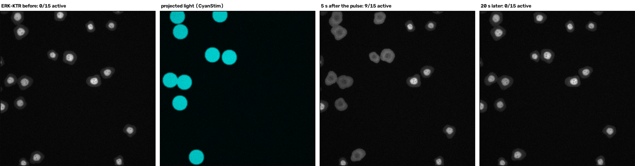
The stimulation light is delivered through the CyanStim channel: a blue LED whose light is shaped by a spatial light modulator (SLM), here a digital micromirror device (DMD). It works like a small projector that switches the stimulation light on or off pixel by pixel; the stimulation mask you compute is uploaded to it.
Why a loop?
Cells move, deform, and respond to the stimulus itself, so a pattern drawn once is soon out of date. And many responses are transient: to keep a cell in a given state, it must be stimulated again and again. In both cases the next stimulation depends on what the sample is doing now, so the microscope has to keep measuring and deciding, in a feedback loop. Passmore et al. (2025) show how this outcome-driven approach can impose artificial cellular states, with the feedback correcting for cell-to-cell heterogeneity and drift over time.
Let’s look at a single optogenetic activation pulse: the ERK response rises, and then decays as the reporter returns to the nucleus. A closed loop can measure each cell’s activity in every cycle and re-stimulate exactly the cells whose activity has dropped, holding them in the active state. Below the traces, crops of the ERK-KTR channel around one cell per condition show the translocation directly (dark nucleus: active):
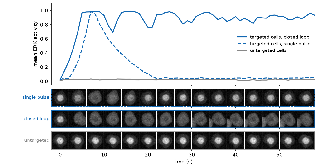
This loop needs no tracking: every cycle detects the nuclei and measures their activity again, and the decision only depends on each cell’s current state. Tracking becomes necessary only when a decision depends on a cell’s history, or when cells must be followed as individuals over time, which is where activity 2 picks up.
Stage 1, image analysis: from pixels to measurements
Every feedback experiment starts with an image-analysis pipeline that extracts data from the live images. Here we use a very basic approach with “classical” image analysis algorithms; in practice this step is often deep-learning based, for example for segmenting cells in label-free images. On a small crop with three cells:
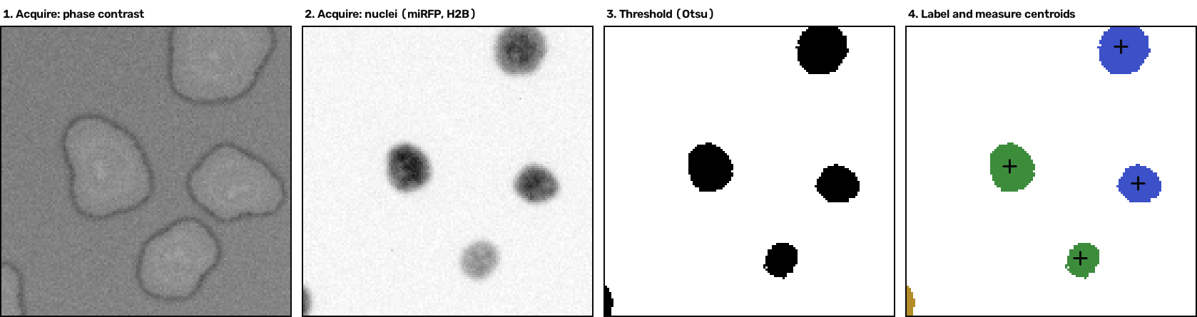
- Acquire the phase-contrast channel (what we display).
- Acquire the nuclear marker channel (
miRFP, what we analyze). Nuclei are compact and never touch, so they stay easy to segment even when cells crowd together. - Threshold the nuclei image. Related module: Thresholding.
- Label connected regions and measure their centroids. Related modules: Connected component labeling, Measure shapes.
Nothing here is specific to smart microscopy, except that it must run fast enough to keep up with the sample.
Stage 2, stimulation logic: from measurements to light
The extracted measurements feed the experiment’s control logic: decide where the light should go, and physically deliver it.
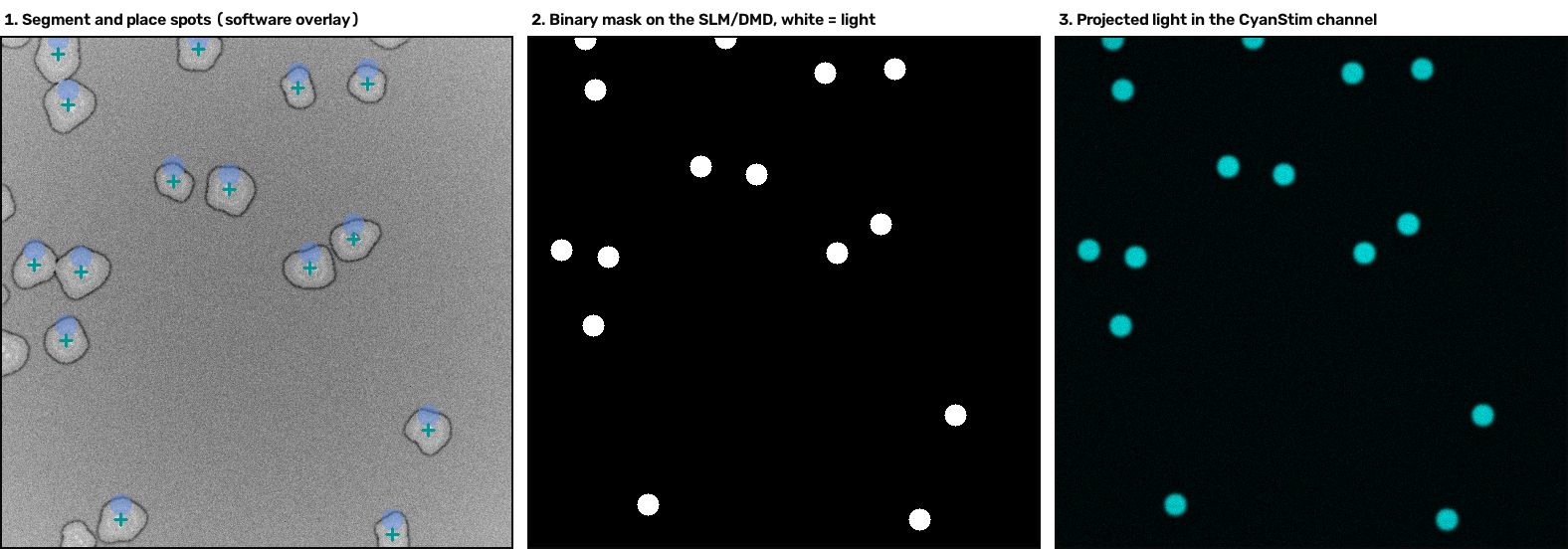
- Decide: turn per-cell measurements into planned illumination spots. Here, the spots are placed above the cell centroids, so that each cell migrates upward.
- Upload: rasterize the plan into a binary mask on the SLM (white = light on). The pattern is loaded, but no light has reached the sample yet, because the SLM only shapes light.
- Deliver: expose in the
CyanStimchannel, i.e. snap with the stimulation light selected. Only now, while the shutter is open, is the pattern projected onto the sample. The camera can image the projected light itself, which is how the alignment between mask and sample is verified on a real system.
A note on timing
The sample does not wait for your software. While an image is being analyzed, the cells keep moving and signaling, so every decision is based on a slightly outdated picture of the sample, and every stimulation lands a little later than planned. Latency and loop frequency are therefore experimental parameters, as real as laser power or exposure time: a slower loop delivers fewer stimuli and acts on older information. The core rule of every feedback experiment: the feedback loop must be faster than the biology it controls. Activity 2 ends with an exploration that makes this failure mode visible.
Activities
Photoactivate a chosen subset of cells
In this first experiment you stimulate a chosen group of cells once and check that exactly these cells respond. It contains all steps of a photomanipulation experiment (image, compute a mask, stimulate, image again) without a loop yet.
- Image the field and detect the cells in the nuclear marker channel
- Check in the biosensor channel that all cells are resting (bright nuclei)
- Choose about half of the cells as targets, by any criterion (position, size, or random), and build a binary stimulation mask with a spot of light on each target
- Stimulate through the stimulation channel, wait a few seconds for the pathway to respond, then image the biosensor channel again
- Check that the targeted cells, and only those, responded (dark nuclei), and quantify it by measuring the activity of every cell before and after the stimulation
- Wait with the light off and check that the response reverses
The expected result is the photoactivation figure in the module introduction, with all cells in the left half of the field as targets.
Then turn it into a closed loop, still without tracking:
- The response decays within tens of seconds, so measure the activity every few seconds and stimulate again exactly the cells whose activity has dropped below a threshold
- The loop needs no cell identities: every cycle detects and measures the cells again, and decides based only on each cell’s current state
- The expected activity traces are shown in the module introduction (single pulse versus closed loop)
Show activity for:
pymmcore-plus (virtual microscope)
Install the simulator once with
pip install "virtual-microscope-teaching[gui]"(Python 3.10 or newer), then run the blocks below one by one, for example as cells of a Jupyter notebook. The next activities continue in the same notebook, with the same microscope and viewer, so the whole module runs top to bottom.Setup
The sample is the
optogeneticsimulation from the setup module: cells expressing optoFGFR (mVenuschannel), ERK-KTR (mScarletchannel) and a nuclear marker (miRFPchannel). In real-time mode the sample keeps changing while your code runs, as on a real microscope, and napari-micromanager shows every snap.channel_layers=Truekeeps one layer per channel, named after it, so that a loop snapping several channels shows all of them, not only the last one.import matplotlib.pyplot as plt import numpy as np from vmteach import load_microscope, run_experiment from vmteach.gui import launch_gui from vmteach.optogenetic import detect_nuclei, measure_activity core, sim = load_microscope("optogenetic", n_cells=20, seed=0, mode="realtime") viewer = launch_gui(core, channel_layers=True)The image analysis uses two small helpers from
vmteach.optogenetic:detect_nuclei()segments the nuclear marker with an Otsu threshold and returns the nucleus centroids, andmeasure_activity()computes each cell’s C/N ratio of the reporter. They are deliberately simple reference implementations, not part of the microscope: they take plain images and return plain lists, so you can replace either of them with your own analysis (for example a deep-learning segmentation), and they work on images from a real microscope as well.Snapping a channel always takes the same three core calls, so wrap them in a small helper:
def snap(channel: str) -> np.ndarray:
    core.setConfig("Channel", channel)
    core.snapImage()
    return core.getImage()
Photoactivation, step by step
The experiment runs in the background with
run_experiment, so the viewer stays live while it runs. The steps are written as one function; the blocks below build it up piece by piece, and the last block runs it.1. Image. Find the cells in the nuclear marker channel, then measure the reporter in the ERK-KTR channel.
measure_activity()computes each cell’s cytoplasm-to-nucleus (C/N) ratio of the reporter and rescales it to 0 (resting) to 1 (fully active). It needs the nuclei image too, to know where each nucleus and its surrounding cytoplasm are.def image_cells(): nuclei = snap("miRFP") cells = detect_nuclei(nuclei) ktr = snap("mScarlet") return cells, ktr, measure_activity(ktr, nuclei, cells)2. Create the mask. Choose who gets light, here every cell in the left half of the field. The mask is a black-and-white image in camera pixels: white means light. A spot of light is a disk of pixels: all pixels closer to its centre than its radius.
yy, xx = np.mgrid[0:512, 0:512]      # row (y) and column (x) of every pixel


def add_spot(mask, x, y, radius):
    """Switch on (255) all mask pixels within radius of (x, y)."""
    mask[(xx - x) ** 2 + (yy - y) ** 2 <= radius ** 2] = 255


def left_half_mask(cells, radius=25):
    targets = [(x, y) for x, y in cells if x < 256]
    mask = np.zeros((512, 512), np.uint8)
    for x, y in targets:
        add_spot(mask, x, y, radius)
    return targets, mask
3. Stimulate. Upload the mask to the SLM and expose with
CyanStim. The snap delivers the light pulse and also records what the projected pattern looks like on the sample.def stimulate(mask): core.setSLMImage("SLM", mask) projected = snap("CyanStim") core.setSLMImage("SLM", np.zeros((512, 512), np.uint8)) return projected4. Put it together. Image, stimulate, wait for the pathway to respond (the full response takes about 5 s), image again, and check once more after 20 s in the dark:
def photoactivation(run):
    cells, ktr_before, before = image_cells()
    targets, mask = left_half_mask(cells)
    projected = stimulate(mask)
    run.sleep(5)
    _, ktr_after, after = image_cells()
    run.sleep(20)
    _, _, later = image_cells()
    return dict(cells=cells, targets=targets, before=before, after=after,
                later=later, ktr_before=ktr_before, projected=projected,
                ktr_after=ktr_after)


run = run_experiment(photoactivation)     # returns immediately
In the viewer, watch the channels update and the nuclei of the targeted cells turn dark in the
mScarletlayer. Note thatimage_cells()detects the cells again each time: they move a little between snaps.Check the result
run.wait()returns what the experiment returned, after about 30 s:res = run.wait() n_active = lambda acts: sum(a > 0.5 for a in acts) print(f"{len(res['cells'])} cells, {len(res['targets'])} targeted, " f"{n_active(res['before'])} active before stimulation") print(f"{n_active(res['after'])} active 5 s after the pulse") print(f"{n_active(res['later'])} active 20 s later") fig, axes = plt.subplots(1, 3, figsize=(12, 4)) for ax, img, title in [(axes[0], res["ktr_before"], "ERK-KTR before"), (axes[1], res["projected"], "projected light (CyanStim)"), (axes[2], res["ktr_after"], "ERK-KTR 5 s after the pulse")]: ax.imshow(img, cmap="gray", vmin=0, vmax=255) ax.set_title(title) ax.axis("off") plt.tight_layout() plt.show()About half of the cells should be targeted, none active before, the targeted ones active after the pulse, and (almost) none active again 20 s later.
Your first closed loop: keep the targeted cells active
A single pulse decays. A loop that measures every second and stimulates again exactly the cells whose activity has dropped keeps them active. No tracking is needed: every cycle detects and measures the cells again, and the decision only depends on each cell’s current position and state.
def keep_active(run, seconds=60, threshold=0.7):
    history = {"targeted": [], "others": []}
    for cycle in range(seconds):
        if run.stop_requested:
            break
        nuclei = snap("miRFP")                               # acquire
        cells = detect_nuclei(nuclei)                        # analyze
        activity = measure_activity(snap("mScarlet"), nuclei, cells)

        mask = np.zeros((512, 512), np.uint8)                # decide
        for (x, y), a in zip(cells, activity):
            if x < 256 and a < threshold:
                add_spot(mask, x, y, 25)

        if mask.any():                                       # actuate
            stimulate(mask)

        left = [a for (x, _), a in zip(cells, activity) if x < 256]
        right = [a for (x, _), a in zip(cells, activity) if x >= 256]
        history["targeted"].append(np.nanmean(left) if left else 0.0)
        history["others"].append(np.nanmean(right) if right else 0.0)
        run.sleep(1.0)
    return history


sim.reset()
history = run_experiment(keep_active).wait()                 # about one minute
Plot the mean activity of both groups over time:
plt.figure(figsize=(7, 3))
plt.plot(history["targeted"], label="targeted cells (kept active by the loop)")
plt.plot(history["others"], label="untargeted cells")
plt.xlabel("time (s)")
plt.ylabel("mean ERK activity")
plt.legend()
plt.tight_layout()
plt.show()
Follow moving targets: the mask must chase the cells
Stimulated cells do not only signal, they also protrude and migrate toward the light. This turns targeted illumination into a way to steer cells, and it brings in the central difficulty of photomanipulation on live samples: the target moves, so a mask computed once is soon out of date. The loop has to recompute the mask from every new image.
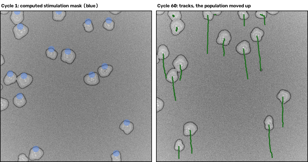
- Run the feedback loop from the previous activity, but place each light spot slightly above its cell instead of on it: every stimulation now pulls the cell upward
- Let the loop run until the whole population has clearly moved up
- Link the per-frame detections into trajectories to see each cell’s path, as in the figure at the top of the module. This is where tracking comes in: the steering decision needs no identities, but following and quantifying each cell’s behavior over time does, because that means keeping cell identities across frames
- Then make the decision per object: steer cells in the left half of the field up and cells in the right half down. Only the decide step changes; acquisition and stimulation stay the same
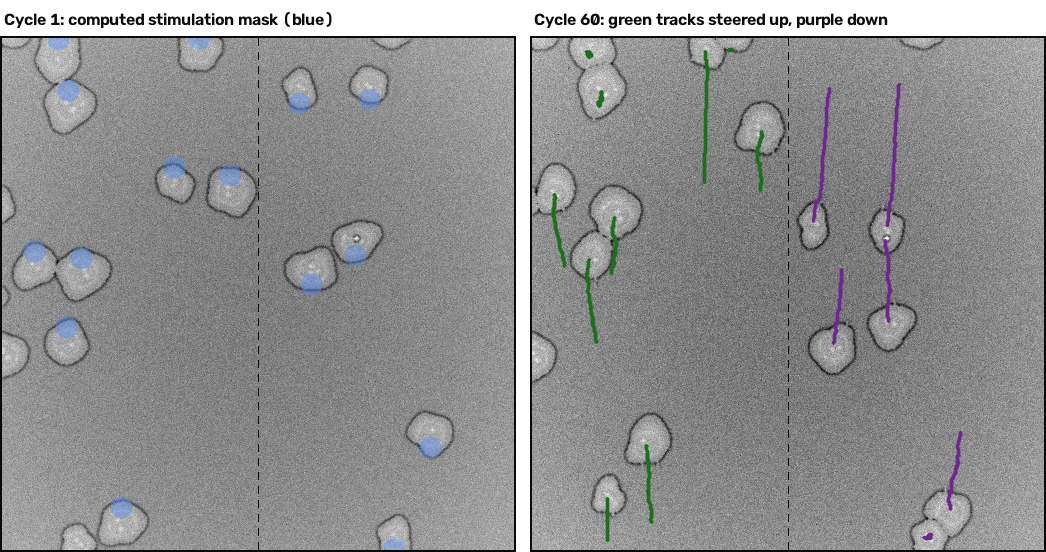
- Explore the loop timing: what happens when the interval between iterations grows?
Show activity for:
pymmcore-plus (virtual microscope)
This continues the notebook of the previous activity:
core,sim,viewer,snap(),add_spot()andstimulate()are already defined, and the microscope keeps running. Run the blocks below one by one.Setup
Stimulated cells protrude and migrate toward the light, so a spot placed slightly above a cell pulls it upward. Because the cells move, the mask must be recomputed from every new image: a feedback loop. Two more helpers are needed:
link_tracksfor tracking, andoverlayto draw a mask on an image.import time from vmteach.gui import show_mask from vmteach.optogenetic import link_tracks, overlayOne pass through the loop
Acquire the nuclear marker channel and detect the cells, with the same pipeline as in the previous activity:
cells = detect_nuclei(snap("miRFP"))
phase = snap("phase-contrast")
print(f"detected {len(cells)} cells")
Decide: one spot per cell, offset upward. The offset direction is the entire steering logic.
def build_steer_mask(cells, dy=-15, spot_radius=11, shape=(512, 512)):
    """One illumination spot per cell, offset by dy pixels in y."""
    mask = np.zeros(shape, dtype=np.uint8)
    for cx, cy in cells:
        add_spot(mask, cx, cy + dy, spot_radius)
    return mask


mask = build_steer_mask(cells)
plt.imshow(overlay(phase, mask))
plt.title("stimulation mask (blue): one spot above each cell")
Actuate with
stimulate()from the previous activity: upload the mask and expose withCyanStim.stimulate(mask)Close the loop
Acquire, analyze, decide, actuate, wait, repeat. Each cycle snaps
miRFPto find the cells and thenCyanStimto deliver the new mask: forget theCyanStimexposure and nothing happens, a classic debugging moment at a real microscope. The loop also snapsphase-contrast, so that you can follow the cells in the viewer, andshow_maskputs the current mask on top, so you can see the spots follow the cells.n_cycles = 60 # one minute def steer_up(run): detections = [] for i in range(n_cycles): if run.stop_requested: break cells = detect_nuclei(snap("miRFP")) # acquire + analyze phase = snap("phase-contrast") # to follow the cells mask = build_steer_mask(cells) # decide stimulate(mask) # actuate show_mask(viewer, mask, "stimulation") detections.append(cells) run.sleep(1.0) # the sample responds return detections, phase sim.reset() run = run_experiment(steer_up) # returns immediatelyThe loop runs in the background, so the notebook stays usable;
run.stop()ends it early. Wait for it to finish:detections, phase = run.wait()Tracking: what did each cell do?
The steering decision never needed cell identities, but following and quantifying each cell over time does.
link_tracks()links the per-frame detections into trajectories (Hungarian assignment with a distance gate); real pipelines use a tracking library such as trackpy.rows = link_tracks(detections) # columns: id, frame, y, x dys = [] for tid in np.unique(rows[:, 0]): tr = rows[rows[:, 0] == tid] if len(tr) >= 10: tr = tr[np.argsort(tr[:, 1])] dys.append(tr[-1, 2] - tr[0, 2]) print(f"{len(dys)} tracks, mean displacement {np.mean(dys):+.0f} px (negative = up)")The mean y position of all nuclei in the first and last frame would not show the movement: the whole population moves, so cells leave the field at the top while new ones enter from below. Displacement along each track does.
Draw the trajectories on the last phase-contrast image of the loop. Use this image and not a new snap: the cells keep moving, and a later image no longer matches the ends of the tracks.
def plot_tracks(rows, color_of, min_len=5):
    """Plot each track as a line (x, y over time), colored by color_of(track)."""
    for tid in np.unique(rows[:, 0]):
        tr = rows[rows[:, 0] == tid]
        if len(tr) < min_len:
            continue
        tr = tr[np.argsort(tr[:, 1])]            # sort by frame
        plt.plot(tr[:, 3], tr[:, 2], color=color_of(tr), lw=2)


plt.imshow(phase, cmap="gray")
plot_tracks(rows, lambda tr: "green")
plt.title("one-minute trajectories: everyone went up")
Per-object decisions
Steer each cell differently based on a measured property: cells left of the midline go up, cells right of it go down. Only the decide step changes; acquisition and actuation stay the same.
def build_split_mask(cells, offset_px=15, spot_radius=11, shape=(512, 512)):
    mask = np.zeros(shape, dtype=np.uint8)
    for cx, cy in cells:
        dy = -offset_px if cx < shape[1] // 2 else +offset_px   # the decision
        add_spot(mask, cx, cy + dy, spot_radius)
    return mask


def steer_split(run):
    detections = []
    for i in range(n_cycles):
        if run.stop_requested:
            break
        cells = detect_nuclei(snap("miRFP"))
        phase = snap("phase-contrast")
        mask = build_split_mask(cells)
        stimulate(mask)
        show_mask(viewer, mask, "stimulation")
        detections.append(cells)
        run.sleep(1.0)
    return detections, phase


sim.reset()
detections, phase = run_experiment(steer_split).wait()
Draw the tracks again, colored by the half of the field each cell started in: green for up, purple for down.
def by_start(tr):
    return "green" if tr[0, 3] < 256 else "purple"


plt.imshow(phase, cmap="gray")
plot_tracks(link_tracks(detections), by_start)
plt.axvline(256, color="w", ls="--")
plt.title("left half steered up, right half steered down")
One measurement per cell, here its x position, is enough to give every cell its own treatment. Any other measured feature works the same way: size, intensity, shape, or biosensor activity.
Explore the timing
The loop timing is the most important parameter of any feedback experiment. Re-run the up-steering loop with
run.sleep(5.0)instead ofrun.sleep(1.0): the same minute now contains five times fewer stimulations, and each mask acts on older information. The steering becomes weaker or fails.The sample keeps moving while your code runs, so the duration of your analysis is part of the experiment too. Add
time.sleep(2)between the analyze and decide steps (a slow segmentation) and watch the spots land where the cells used to be. This is exactly the situation on a real microscope.
Exercise: assemble the cells into a letter
In the previous activities you steered all cells in a fixed direction. Now use the same feedback loop to make the cells assemble into a target shape, a letter of your choice. The exercise is modelled after the letter-assembly experiments of Hinderling et al. (2025), where we guided fibroblasts into letter-shaped patterns over several days. This is an open design problem: there is no single correct solution, and iterating toward one that works is the point of the exercise.
- Create a binary target image of a letter and display it on top of a snapped image
- Segment the cells. Tip: as cells crowd together on the letter, their bodies touch and merge under a simple threshold. Segment the nuclei instead: they stay separated because cells collide before their nuclei can touch, which is also why real workflows often segment nuclei rather than cell bodies
- Design a decision rule that steers each cell toward the letter, and run it in the feedback loop until the letter forms
- Quantify success. Two candidate metrics; which is fairer, and why?
- fraction of target pixels covered by cells
- fraction of cells whose centroid is on the target
With a working strategy, the population assembles into a clearly legible letter; perfect filling is impossible, see the questions below:
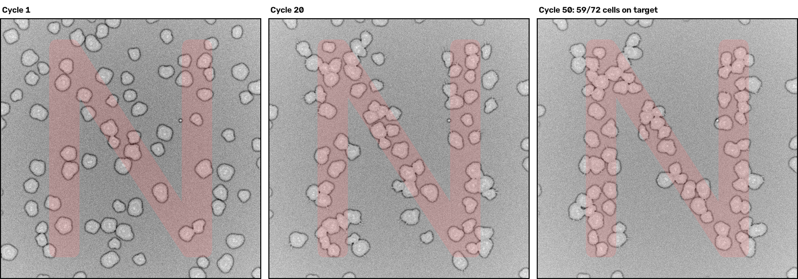
The implementation tab below provides the setup, a ladder of hints (read them one at a time, only when stuck), and a validated reference solution.
Going further (optional):
- Why can pixel coverage never reach 100%, even when most cells are on the letter? Think about the minimal distance between two cells, then look at the sharp corners of the letter, where crowding is worst
- Pick a letter with disconnected parts or enclosed holes (“i”, “O”). Which parts of your strategy break, and why?
- Log your metric every cycle and plot it over time. Where does the strategy spend most of its time: recruiting distant cells, or resolving traffic jams?
- Make the rules state-dependent: once most positions are filled, switch to a “maintenance mode” that pushes surplus cells away from the letter so they stop crowding its boundary
Show activity for:
pymmcore-plus (virtual microscope)
This continues the notebook of the previous activities:
core,sim,viewer,snap(),add_spot()andstimulate()are already defined, and the microscope keeps running.Setup
from scipy import ndimage
from scipy.spatial import cKDTree
from vmteach.optogenetic import letter_mask

sim.reset(n_cells=75, base_radius=13.0)   # smaller, more numerous cells
SPEED = 5                                 # simulation only: 5x faster than real time
sim.speed = SPEED
target = letter_mask("N", fill=0.85, thickness=60)   # uint8, 255 inside the letter
show_mask(viewer, target, "target", color="orange")  # overlay in the viewer
sim.reset()rebuilds the population on the running microscope: smaller and more numerous cells than in the earlier activities, because cells are solid objects that need room on the stroke of the letter.Real cells need minutes to assemble, and every attempt at a real microscope costs that long. A simulation can simply run faster: with
sim.speed = SPEEDthe sample evolves five times faster than in real time, so wait1.0 / SPEEDseconds per cycle to keep one second of cell time per cycle. About 50 cycles are enough for the letter to form, which takes 10 s instead of 50 s. On a real microscopeSPEEDis 1 and the rest of your script stays the same. One thing does not speed up: your own code. AtSPEED = 5, 30 ms of analysis cost 0.15 s of cell behavior, so the information each mask acts on is proportionally older.Hint 1: what should each cell do?
Treat each cell independently, exactly like in the split-steering activity: for every detected cell, decide where its illumination spot should go. A cell moves toward its spot, so aim each cell at a target pixel, and stop stimulating it once it has arrived.
Hint 2: finding the nearest target pixel
scipy.spatial.cKDTreeon the target coordinates does this in two lines:from scipy.spatial import cKDTree target_pts = np.column_stack(np.nonzero(target)[::-1]) # (x, y) pairs tree = cKDTree(target_pts) dist, idx = tree.query([(cx, cy) for cx, cy in cells])Two catches, both worth discovering yourself first:
- Don’t place the spot on the possibly distant target pixel, because the cell only responds to light near its own body. Place the spot a fixed step (about 12 px) from the cell centroid, in the direction of the target pixel.
- The nearest target pixel is always on the letter’s edge. A cell that stops there is half outside. Aim at the stroke’s core instead:
ndimage.distance_transform_edt(target > 0)gives each letter pixel’s distance to the letter edge, and pixels with distance of 14 or more are “deep”. Use those as the routing targets, and consider a cell “arrived” when its centroid reaches a deep pixel.Hint 3: my cells pile up and block each other!
Two crowd-control problems appear, both real issues in tissue-patterning experiments:
- Everyone heads to the same spot. Remove target pixels that are already claimed by a cell before the nearest-pixel query, so free cells are routed to unoccupied parts of the letter.
- The removal radius must respect cell spacing. The simulated cells collide (and stop) when their centers come within roughly two cell radii (~28 px for
base_radius=13). If you only remove a small disc around each settled cell, the next cell aims at a pixel directly beside an occupied one and gets blocked by the collision. Remove a disc of about the collision distance (~28 px) so every routing target is a spot where a cell can actually fit.Solution
Validated reference solution (50 cycles, about 10 s at
SPEED = 5). Expect roughly 80 to 90% of the detected cells to settle on the target, forming a clearly legible letter as in the expected progression shown above, while pixel coverage stays around 40%. Perfect filling is not achievable, see the “Going further” questions.dist_in = ndimage.distance_transform_edt(target > 0) DEEP = 14 # "core" of the letter stroke deep = (dist_in >= DEEP).astype(np.uint8) * 255 deep_pts_all = np.column_stack(np.nonzero(deep)[::-1]) def build_letter_mask(cells, step_px=12, spot_r=11, occupied_r=28, shape=(512, 512)): mask = np.zeros(shape, np.uint8) # routing targets: unoccupied core pixels, with cell-sized spacing free_deep = deep.copy() for cx, cy in cells: free_deep[(xx - cx) ** 2 + (yy - cy) ** 2 <= occupied_r ** 2] = 0 pts = np.column_stack(np.nonzero(free_deep)[::-1]) if len(pts) == 0: # letter full, stop recruiting pts = deep_pts_all tree = cKDTree(pts) for cx, cy in cells: if dist_in[cy, cx] >= DEEP: continue # settled: no stimulus, stays put _, i = tree.query((cx, cy)) vx, vy = pts[i] - (cx, cy) d = np.hypot(vx, vy) if d == 0: continue s = min(step_px, d) add_spot(mask, cx + s * vx / d, cy + s * vy / d, spot_r) return mask def assemble(run): for i in range(50): if run.stop_requested: break cells = detect_nuclei(snap("miRFP")) # acquire nuclei snap("phase-contrast") # to follow the cells mask = build_letter_mask(cells) stimulate(mask) # expose the pattern show_mask(viewer, mask, "stimulation") run.sleep(1.0 / SPEED) # one second of cell time return cells, snap("mScarlet") # filled cell bodies for the metric sim.reset() cells, img = run_experiment(assemble).wait() # watch the letter form liveMetrics:
def otsu_threshold(img):
    """The gray level that best separates dark from bright pixels (Otsu)."""
    p = np.bincount(img.ravel(), minlength=256) / img.size
    w = np.cumsum(p)                             # fraction of pixels below
    mu = np.cumsum(p * np.arange(256))           # their summed intensity
    between = (mu[-1] * w - mu) ** 2 / np.maximum(w * (1 - w), 1e-12)
    return np.argmax(between)

# the mScarlet reporter fills the whole cell body, so a threshold on it
# gives a cell-pixel mask for the coverage metric
cell_px = img > otsu_threshold(img)
coverage = (cell_px & (target > 0)).sum() / (target > 0).sum()
on_target = sum(1 for cx, cy in cells if target[cy, cx] > 0) / len(cells)
print(f"target coverage {coverage:.0%}, cells on target {on_target:.0%}")
The cells on target fraction is the fairer metric: pixel coverage can never reach 100% because the cells keep a collision distance. Like real cells, they cannot be packed arbitrarily densely.
Explore the finished experiment in napari (
vmteach.gui.show_results): overlay the stimulation masks and tracks to see exactly where your routing sent each cell. Tracking usesvmteach.optogenetic.link_tracks, a short Hungarian assignment with distance gating. On real data you would reach for a tracking library with the same detections-in, tracks-out interface: trackpy, btrack, or motile.
Assessment
Scenario checks
- You run the steering experiment and the cells do not move. Name three different places the experiment can silently fail, and for each, one extra image or measurement that would expose it.
Solution
Any three of, for example: the analysis finds no or wrong cells (overlay the detections on the image); the mask is computed in the wrong place or coordinates (display the mask on top of the image); the light is never delivered, for example the stimulation channel is selected but never exposed (image the projected light and check it matches the mask); the light lands but the response is too weak or the sample does not respond (check a single cell with a strong manual stimulus). The habit to build: make every stage of the loop inspectable.
- An experiment stimulates the same hand-drawn region every 30 seconds for an hour. Give one experiment where this open-loop design is perfectly fine, and one where it quietly produces garbage.
Solution
Fine: the target does not move or respond, for example bleaching a region of a fixed sample, or activating a spot in a dish where position does not matter. Garbage: anything where the target moves, deforms, or reacts, for example migrating cells leave the region within minutes, so later pulses hit the wrong cells while the experiment looks like it is running normally.
- Between snapping an image and the light reaching the sample, the sample has changed. What two properties of your experiment decide whether this matters?
Solution
How fast the sample changes relative to the loop’s latency, and how spatially precise the stimulation must be. A slow-moving cell hit by a generous spot tolerates seconds of delay; a subcellular target on a fast-moving edge does not. This is why latency is an experimental parameter, not an implementation detail.
- For each goal, decide whether the loop needs to keep cell identities across frames, and why: (a) keep every cell in the field active; (b) stimulate each cell exactly three times; (c) stimulate only cells that have been quiet for the last five minutes; (d) steer all cells to the left.
Solution
(a) No: re-detect and re-measure each cycle, the decision depends only on each cell’s current state. (b) Yes: “three times” is per-cell history, so cells must be recognized across frames. (c) Yes: “quiet for five minutes” is also history. (d) No: every detected cell gets the same treatment each cycle. The rule: tracking is needed exactly when a decision depends on a cell’s past, not only on its present.
- Now imagine the cells had no ERK activity reporter, only the nuclear marker. Which experiments from this module still work, and which require ERK-KTR?
Solution
The steering and letter experiments still work: their readout is position, which the nuclear marker provides. The photoactivation and keep-active experiments need ERK-KTR: without an activity readout, stimulation is still delivered, but nothing in the images reports whether the pathway responded, so the loop cannot verify or regulate activity.
- The activities use two image analysis helpers,
detect_nuclei(img)andmeasure_activity(ktr_img, nuclei_img, centroids). You want to replace them with your own, for example a deep-learning segmentation. What does each function take as input and return as output, so that the rest of the loop keeps working unchanged? And when would a centroid per cell not be enough?
Solution
detect_nucleitakes one image of the nuclear marker channel (a 2D array) and returns one(x, y)centroid per nucleus, in camera pixels.measure_activitytakes the reporter image, the nuclear marker image of the same field and those centroids, and returns one number per centroid, in the same order: the activity between 0 (resting) and 1 (fully active), ornanwhere it could not be measured. Any replacement with the same inputs and outputs fits into the loop.Centroids are enough for everything in this module: placing a spot at an offset from the nucleus, and tracking. Other stimulation strategies need the whole segmentation, for example stimulating the edge of each cell rather than a spot next to its nucleus, or illuminating the entire cell body. A replacement should then return a label image (one integer per cell, 0 for background), from which centroids, outlines and edges can all be derived.
The versions used in the activities, condensed from
vmteach.optogeneticand written with numpy andscipy.ndimage:import numpy as np from scipy import ndimage def otsu_threshold(img): """The gray level that best separates dark from bright pixels (Otsu).""" p = np.bincount(img.ravel(), minlength=256) / img.size w = np.cumsum(p) # fraction of pixels below mu = np.cumsum(p * np.arange(256)) # their summed intensity between = (mu[-1] * w - mu) ** 2 / np.maximum(w * (1 - w), 1e-12) return np.argmax(between) def label_nuclei(img): """Label image: threshold, then number the connected bright regions.""" labels, _ = ndimage.label(img > otsu_threshold(img), structure=np.ones((3, 3))) return labels def detect_nuclei(img, min_area=20): """Nucleus centroids (x, y), without small specks and clipped nuclei.""" labels = label_nuclei(img) h, w = img.shape centroids = [] for i, (sy, sx) in enumerate(ndimage.find_objects(labels), start=1): ys, xs = np.nonzero(labels[sy, sx] == i) if len(ys) < min_area: continue # noise if sy.start == 0 or sx.start == 0 or sy.stop == h or sx.stop == w: continue # cut off by the border centroids.append((int(xs.mean()) + sx.start, int(ys.mean()) + sy.start)) return centroids def measure_activity(ktr_img, nuclei_img, centroids, lo=0.3, hi=1.2): """C/N ratio of the reporter per cell, rescaled to 0 (lo) .. 1 (hi).""" labels = label_nuclei(nuclei_img) img = ktr_img.astype(float) bg = np.percentile(img, 5) # camera background r = np.arange(-4, 5) disk = lambda radius: r[:, None] ** 2 + r[None, :] ** 2 <= radius ** 2 activity = [] for x, y in centroids: if labels[y, x] == 0: # centroid not on a nucleus activity.append(np.nan) continue nucleus = labels == labels[y, x] inside = ndimage.binary_erosion(nucleus, disk(1)) ring = (ndimage.binary_dilation(nucleus, disk(4)) & ~ndimage.binary_dilation(nucleus, disk(1))) ring &= (labels == 0) & (img > bg + 8) # cytoplasm, not background n = np.median(img[inside]) - bg c = np.median(img[ring]) - bg activity.append(np.clip((c / max(n, 1) - lo) / (hi - lo), 0, 1)) return activityThe C/N ratio does not depend on how bright a cell is, which is why it is the standard readout of translocation reporters. On real data, calibrate
loandhifrom resting and maximally stimulated control cells.
Discuss with your neighbour
- For which photomanipulation experiments would an open-loop (pre-defined pattern) approach be sufficient, and where is feedback strictly required?
- What could you measure during the experiment to detect that your feedback loop is failing (segmentation errors, cells not responding)?
- Sketch a feedback experiment for your own project: what would the microscope measure, what would it decide, and what would it change on the sample? What is the fastest-changing thing in your sample, and what loop speed does that dictate?
- A feedback experiment makes decisions while you are at lunch. What would you log during the run so that you can trust the result afterwards?
Follow-up material
Recommended follow-up modules:
Learn more:
SMWG white paper: Smart microscopy, current implementations and a roadmap for interoperability
FARO: Real-time feedback control microscopy for automation of optogenetic targeting
Smart Microscopy Exercise (H. Heil): analysis-driven targeted acquisition on real data
virtual-microscope-teaching: the simulator used in this module